


The procedure for defining adaptive meshing is as follows:
In the task menu, select the Numerical parameters menu item.
 Numerical parameters
In the Numerical parameters menu, select Adaptive meshing.
Adaptive meshing
Enable the appropriate type of meshing by selecting the corresponding item in the Adaptive Meshing menu:
For problems involving internal moving parts (that is, that use the MST), select Activate adaptive meshing for moving parts.
Activate adaptive meshing for moving parts
For problems involving species transport, and big variations of fields on fixed meshes, select Activate adaptive meshing for large variations of fields.
Activate adaptive meshing for large variations of
fields
For problems involving shell blow molding (contact), select Activate adaptive meshing for contacts.
Activate adaptive meshing for contacts
For all other blow molding simulations, select both Activate adaptive meshing for contacts and Activate adaptive meshing for remeshings.
Activate adaptive meshing for contacts
Activate adaptive meshing for remeshings
Activate adaptive meshing for remeshings is available only if you are using the Thompson, Lagrangian, elastic, or improved elastic remeshing method.
Set the parameters for the type of adaptive meshing you have selected.
Select Upper level menu to return to the Adaptive Meshing menu.
Set the general adaptive meshing parameters.
Specify the frequency of the meshing.
Modify Nstep
A value of 1 (the default) indicates that the adaptive meshing will be performed at each time step. This value is appropriate for MST simulations, because the fluid region is changing significantly from one time step to the next. A value of 3 is good for species transport simulations.
For simulations involving large variations on fixed mesh, a value of 1 might be necessary to assume good convergence scheme. A value of 5 (the default for contact with shells) is usually sufficient for contact and remeshing simulations.
For transient simulations using triangular / tetrahedral element generation, a value smaller than 4 does not allow for an appropriate estimation of the time step, so that it will not be adapted with predictor-corrector scheme. The time step remains constant through out the simulation but can be reduced if the solution does not converge.
For blow molding, thermoforming applications, as well as pressing applications, the parameter NStep is set to 5 by default. This appears to be a good compromise for enabling the selection of appropriate time steps while guaranteeing acceptable element distortion.
Note: A reliable alternative is to remesh every 4 or 5 time steps and to invoke the element distortion check.
Specify the number of times a primitive element (that is, an element of the initial mesh, as created in the mesh generator) can be subdivided recursively.
Modify Maxdiv
A value of 3 (the default) means that a given 2D surface of area
 :
: will have 4 subfaces of area
 after one subdivision
 can have up to 16 subfaces of area
 after two subdivisions
 can have up to 64 subfaces of area
 after three subdivisions
Because different subdivision methods can be used for shells (the specific method is automatically selected by the solver to maximize the quality of generated sub-elements), a value of 3 (the default) means that a given shell surface of area
 :
:will have 2 subfaces of area
 or 4 subfaces of area
  after one subdivision
can have between 4 subfaces of area
 to 16 subfaces of area
  after two subdivisions
can have between 8 subfaces of area
 to 64 subfaces of area
  after three subdivisions
A value of 3 (the default) also means that given brick of volume
 :
: will have 8 sub-bricks of volume
 after one subdivision
 can have up to 64 sub-bricks of volume
 after two subdivisions
 can have up to 512 sub-bricks of volume
 after three subdivisions
A value greater than 3 will lead to a large increase in the number of elements. For 3D, a maximum value of 2 is recommended.
Enable partial triangulation 3D.
Remeshing with triangular / tetrahedral element generation depends on criteria that select elements to remesh. If Full triangulation is used, when one element is selected for remeshing, the whole moving domain (that is, the domain for which there are local criteria activated) will be remeshed. With big meshes, the cost of this operation could be too high.
A better solution is the Partial Triangulation 3D. When one element is selected for remeshing, a zone defined upon the neighbors of this element will be remeshed (and not the entire mesh). This option is preferable for large meshes.
For 2D and shell meshes that use the recursive subdivision technique, you can enable conformalization for the mesh.
Enable Mesh Conformalization
The conformalization takes place after the subdivision; it ensures that the mesh only contains conformal elements (see Figure 16.17: Example of Conformalization) and eliminates all the constraints that are needed to guarantee the continuity of the fields for midsegment nodes. Mesh conformalization is enabled by default for blow molding and thermoforming simulations that involve adaptive meshing in the setup. In other cases, conformalization is optional.
Conformalization is useful in the following circumstances: when your postprocessor does not support or does not correctly handle non-conformal meshes; when you want to avoid the wiggles that can appear in the solution when contact is establishing; when you want to avoid the conflict that can arise between constraints of conformity and other constraints (for example, those created for fluid-solid contact handling and connected boundaries).
Note that conformalization can also be applied on existing non-conformal meshes, as described in Converting a Shell Mesh and Results.
For blow molding and thermoforming simulations that involve both contact and adaptive meshing, you can specify that an additional adaptive meshing step is performed before the start of the transient simulation. Note that for blow molding simulations, contact problems on a shell mesh will involve adaptive meshing by recursive subdivision if Lagrangian remeshing is enabled; for thermoforming simulations, contact problems will involve adaptive meshing by triangular / tetrahedral element generation if Thompson, Lagrangian, elastic, or improved elastic remeshing is enabled.
Enable additional adaptive meshing at start
If the surface of the fluid in its initial position is close to the surface of contact of the mold, it is possible that contact can occur before the first remeshing of the transient simulation (which you scheduled using the Modify Nstep menu item). In such cases, it can be useful to remesh before starting the transient simulation, so that the fluid elements are refined near the finer details of the mold, and can therefore conform more closely to the shape of the mold.
If you want to reset the frequency and number of subdivisions and the Partial/Full triangulation switch to the default values, select Reset parameters of adaptive meshing (to default values).
For adaptive meshing with moving parts, you can specify the moving parts for which adaptive meshing should be performed. You can also specify different adaptive meshing parameters for each of the moving parts, or specify a single set of parameters that apply to all of them.
When you select Activate adaptive meshing for moving parts, as described above, you will enter the Global criteria for moving parts menu, where you can follow the steps below to set the relevant parameters:
To enable adaptive meshing for all of the moving parts, select Enable all the local criteria.
Enable all the local criteria
If you want to enable (or disable) adaptive meshing for one or more individual parts, select the Criteria on menu item for the relevant part, select Enable current criteria (or Disable current criteria) in the Local criteria for moving parts menu, and then select Upper level menu to return to the Global criteria for moving parts menu.
Set the global parameters for meshing,
 and
and  , as described below.
Modify S_up
Modify S_do
, as described below.
Modify S_up
Modify S_do
Each time you modify the value of a global parameter, it will be used for all enabled local criteria.
In the mesh superposition technique, each node in the flow domain is evaluated to determine if it lies in the real fluid region or in a moving part. This information is stored in a field called the "inside" field. At each nodal point, if the value of the inside field is 0, the point is in the fluid region; otherwise, its value is 1. In order to better represent the exact shape of the moving part by the inside field, the mesh must be refined in the neighborhood of the moving part's border.
The border of a moving part can be identified as the region of the flow domain where the gradient of the inside field is nonzero. Thus, with the default method using the variation of inside field, the criteria for adaptive meshing are as follows:
If the variation of the inside field across an element is greater than
 , the element is subdivided. The default value
for
, the element is subdivided. The default value
for  is 0.05.
 If the variation of the inside field across an element is less than
 , the element is unrefined (coarsened). The
default value for
, the element is unrefined (coarsened). The
default value for  is 0.01.
 If the simulation is transient, then as a moving part rotates, all of the elements in the flow region will come into contact with its border, and they will therefore be subdivided. As the part moves away, these additional subelements are no longer necessary, and their presence will lead to an increase in CPU time and memory usage. To avoid this problem, Ansys Polyflow will remove the subelements in the areas distant from the borders of the moving part.
If you want to return to the default global values of
 and
and  , select Reset global parameters (to default
values).
, select Reset global parameters (to default
values). Specify the mesh adaption method.
Switch to calculated from variation of inside field
(default)or
Switch to calculated from average of inside field
There are two methods that Ansys Polyflow can use to select elements for remeshing; Variation of inside field and Average of inside field. Both of these methods refine or "un-refine" the mesh based on whether the returned value is above
 or below
  . Variation of inside field adapts
the mesh based on the variation of the value of inside
field across the element. Average of inside
field adapts the mesh based on the average value of
inside field across the element.
Average of inside field also refines on the
border and inside the moving parts, which makes it more computationally
expensive, but yields better results. Choose Average of inside
field if you observe mass loss and/or anomalies in
velocity fields using Variation of inside
fields.
. Variation of inside field adapts
the mesh based on the variation of the value of inside
field across the element. Average of inside
field adapts the mesh based on the average value of
inside field across the element.
Average of inside field also refines on the
border and inside the moving parts, which makes it more computationally
expensive, but yields better results. Choose Average of inside
field if you observe mass loss and/or anomalies in
velocity fields using Variation of inside
fields.To enable or disable local criteria for a specific moving part, click the Criteria on [moving part #xx] menu item for the relevant part.
If you want to modify the
 and
and  values for a particular moving part, click
Switch to ‘Local Criteria’ mode.
Once you are in Local criteria mode, you no longer
have access to the global parameters. Clicking the Criteria on
[moving part #xx] menu item opens the Local
criteria for moving parts menu, which allows you to
define the
values for a particular moving part, click
Switch to ‘Local Criteria’ mode.
Once you are in Local criteria mode, you no longer
have access to the global parameters. Clicking the Criteria on
[moving part #xx] menu item opens the Local
criteria for moving parts menu, which allows you to
define the  and
and  for the current sub-part. If you want to copy the
global values of
for the current sub-part. If you want to copy the
global values of  and
and  to this moving part, select Reset local
parameters (copy global param.).
to this moving part, select Reset local
parameters (copy global param.).
For transport of species simulations, the local meshing criteria are defined and you can choose to activate or deactivate them. For the adaptive meshing for large variations of fields, you must define your own local criteria for the remeshing. The procedure is as follows:
Click Add Local Criteria for refinement.
Select the field for which you want to define a criteria. The fields available depend on the type of the simulation you do.
For generalized Newtonian flows:
Normalized velocity
Each component of the velocity
Temperature (if non isothermal flow)
Local shear rate (if postprocessor defined)
For Darcy flow problems:
Pressure Darcy
For electrical potential problems:
Potential
For viscoelastic flows:
First invariant of tensions
Second invariant of tensions
Choose the domains you want to remesh. You can choose from the list of domains available for each field selected.
Repeat steps 2 and 3 if you want to add another refinement for another field.
Note: When a local criterion is defined, you cannot remove it from the list but only deactivate it.
Once you click Upper level menu Ansys Polydata returns to the Global criteria for large variations of fields menu. You can see the criteria you have defined in the list of Local Criteria.
In the Global criteria for large variations for fields
menu, you can modify the  and
and  values that will be used for all local criteria.
Clicking Reset global parameters (to default values) will
reset  and
and  to default values for all local criteria.
All local criteria can be disabled/enabled by clicking Disable/Enable all the local criteria.
If you want to disable/enable a specific refinement, click the Criteria on [Refinement for...] menu item for the corresponding field.
To define different  and
and  values for the different fields, click Switch to
‘Local Criteria’ mode. Once you are in
Local criteria mode, you no longer have access to the
global parameters. Clicking the Criteria on [Refinement
for...] menu item for a specific field opens the Local
criteria for large variations of field menu, where you can
enable/disable the current refinement, set the local
values for the different fields, click Switch to
‘Local Criteria’ mode. Once you are in
Local criteria mode, you no longer have access to the
global parameters. Clicking the Criteria on [Refinement
for...] menu item for a specific field opens the Local
criteria for large variations of field menu, where you can
enable/disable the current refinement, set the local  and
and  parameters or reset them to the value of the global
parameters.
parameters or reset them to the value of the global
parameters.
For blow molding and thermoforming simulations, which involve both a contact problem and remeshing for the parison / preform / sheet deformation over time, you will specify two groups of parameters for adaptive meshing: one for the contact (as described in Adaptive Meshing for Contact), and one for the standard remeshing (as described in Adaptive Meshing for Remeshing).
For the contact problem, adaptive meshing can be used to refine the mesh in regions of the fluid that are close to the mold. The meshing calculation can be based on one of the following:
distance
This meshing method refines the fluid mesh using a multi-ramp function of the distance to the mold. This method is recommended when you want to refine the mesh in the boundary layer for problems where there is heat transfer between the fluid and the mold, for example. Note that if you want to have the fluid mesh conform closely to the shape of a mold with fine details, the element count for the fluid mesh will be relatively high.
This method is available for 2D, 3D, and shell elements.
curvature
For this meshing method, the fluid mesh can be refined as it approaches the mold in one of two ways. In the first option, the refinement can be based on the local curvature of the mold elements. This option can produce a fluid mesh that conforms closely with the shape of a mold with fine details, and the element count of the fluid mesh will be lower than that produced by the distance-based remeshing method; however, this option requires that the elements of the mold be relatively small and consistent in size, in order to ensure that the local curvature always accurately represents the shape of the mold. In the second option, the fluid mesh is refined to a specified size wherever it comes into contact with the mold, in a similar manner to the distance-based remeshing method. For both options, the fluid mesh is also refined according to a second-order polynomial function of the distance to the mold.
This method is available for 2D, 3D, and shell elements.
angle and curvature
This meshing method refines the fluid mesh as it approaches the mold, based on either the angle between neighboring mold elements or the local curvature of the mold elements (whichever produces a more refined mesh). This method can produce a fluid mesh that conforms closely with the shape of a mold with fine details, without the limitations of the distance- or curvature-based remeshing methods: the element count of the fluid mesh will be relatively low, and the elements of the mold can be larger and more inconsistent in size.
Important: This method is only available for shell elements.
To specify the settings that determine how the fluid mesh is refined as it approaches the mold, click the Activate adaptive meshing for contacts menu item.
![]() Activate adaptive meshing for contacts
Activate adaptive meshing for contacts
In the Global criteria for contact menu that opens, perform the steps in the following sections, based on the meshing method that is appropriate for your problem.
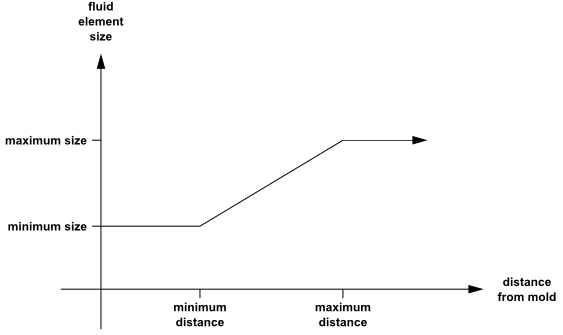
When the fluid elements are refined based on their distance to the
mold surface, you have to define a multi-ramp function by specifying the
minimum size, minimum distance, maximum size, and maximum distance
(Figure 16.18: Multi-Ramp Function for Fluid Element Size). For a given element that
is located a distance  from the mold wall, the minimum size is applied if
 is lower than the minimum distance. If
  is greater than the maximum distance, then the maximum
size is applied. If
is greater than the maximum distance, then the maximum
size is applied. If  is between the minimum and maximum distances, a linear
interpolation between the minimum and maximum sizes is applied.
is between the minimum and maximum distances, a linear
interpolation between the minimum and maximum sizes is applied.
Note: When you invoke the adaptive meshing based on distance to the mold surface, the distance is actually evaluated with respect to the nodes of the mold surface. It is a good practice rule, therefore, to have mold elements whose size does not differ too much from that of the fluid elements. Often, the geometry of the mold will be such that the elements will already have a reasonable size. In exceptional situations, however, where the mold is geometrically simple (such as a flat surface), care should be taken for the element size.
To specify that the meshing calculation is based on distance, click the following in the Global criteria for contact menu:
![]() Switch to calculated from distance
Switch to calculated from distance
To begin the setup, enable the adaptive meshing for one or more contact boundaries using the procedure described for moving parts (see Adaptive Meshing Parameters for Moving Parts).
Next, modify the following parameters:
-
Modify size_min
This sets the minimum size for elements close to the mold boundary.
-
Modify dist_min
This sets the minimum distance below which the minimum size is applied.
-
Modify size_max
This sets the maximum size for elements far from the mold boundary.
-
Modify dist_max
This sets the maximum distance beyond which the maximum size is applied.
When the meshing is based on the local curvature of the mold, the
behavior can be modeled mathematically as follows. For a given element
 of the parison / preform / sheet, with a size
 , Ansys Polyflow searches for the closest node
 of the mold. The distance between element
 and node
  is denoted as
  , and the local radius of curvature at node
 is denoted as
  . Element
  will be refined if its proposed new size
 is less than
  , where the new size is computed from
 | (16–21) |
where  is the fraction of the radius of curvature,
 is the desired size of element
  when
when  is in contact with the mold,
  is the typical distance to the mold,
  is a coefficient of proportionality, and
 is the minimum size for an element in the fluid.
Refinement begins when the distance
is the minimum size for an element in the fluid.
Refinement begins when the distance  between element
  and the mold is less than
  . Defining the parameters allows you to modulate the
refinement along the free surface.
. Defining the parameters allows you to modulate the
refinement along the free surface.  may be interpreted as the intended size of the fluid
elements when the contact occurs along a flat part of the mold. There
are two extreme scenarios:
may be interpreted as the intended size of the fluid
elements when the contact occurs along a flat part of the mold. There
are two extreme scenarios:
 and
and 
These values should be used when the contact occurs along a flat part of the mold.
 and
and 
These values are recommended for contact that occurs along a curved mold.
Nonzero values for both parameters  and
and  must be avoided or used very carefully. If the contact
occurs along a flat part of the mold,
must be avoided or used very carefully. If the contact
occurs along a flat part of the mold,  is very large and
  is even larger, and hence, the new size will never be
smaller than the current size.
is even larger, and hence, the new size will never be
smaller than the current size.
To specify that the meshing calculation is based on the local curvature of the mold, click the following in the Global criteria for contact menu:
![]() Switch to calculated from curvature
Switch to calculated from curvature
To begin the setup, enable the adaptive meshing for one or more contact boundaries using the procedure described for moving parts (see Adaptive Meshing Parameters for Moving Parts).
Then you can specify the values of the parameters  ,
,  ,
,  , and
, and  from Equation 16–21
using the following menu items.
from Equation 16–21
using the following menu items.
![]() Modify A
Modify A
![]() Modify B
Modify B
![]() Modify C
Modify C
![]() Modify size_min
Modify size_min
The parameter  is dimensionless, and its default value is 0.2. This
value should lead to almost 30 elements to mesh a circle. The parameters
is dimensionless, and its default value is 0.2. This
value should lead to almost 30 elements to mesh a circle. The parameters
 and
and  have units of length. The default value for
 is the typical size of segments of the mesh, whereas
for
is the typical size of segments of the mesh, whereas
for  it is zero. The parameter
  also has units of length, and its default value is 10%
of the typical size of the segments in the mesh.
also has units of length, and its default value is 10%
of the typical size of the segments in the mesh.
This method is the default for contact with shells.
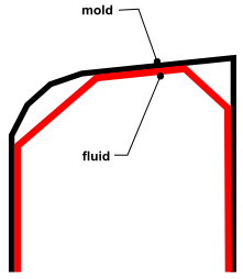
To understand this meshing method, consider a discretized sheet of fluid that completely contacts the mold, that is, the distance between the vertices of the sheet of fluid and the surface of the mold is 0. Under certain circumstances, the nodes in curved or angular portions of the mold can be separated from the centers of the nearest fluid elements by a nonvanishing distance, as shown in Figure 16.19: Contact Between Fluid and Mold. You can specify that the fluid elements are refined in these areas, so that this nonvanishing distance reduces to a more appropriate value.
As part of this meshing method, you specify a tolerance
 , that is, the maximum distance you would ideally like
between any node of the mold and the nearest fluid element. This
tolerance is used to calculate a quantity denoted as
, that is, the maximum distance you would ideally like
between any node of the mold and the nearest fluid element. This
tolerance is used to calculate a quantity denoted as  for each mold node, which represents a fluid element
size that is ideal, in that it could approach the node within the stated
tolerance.
for each mold node, which represents a fluid element
size that is ideal, in that it could approach the node within the stated
tolerance.
Two methods are used to generate  : one based on the angle of the mold elements at the
node, and another based on the local curvature of the mold elements
surrounding the node. The lesser of these two values is selected, in
order to ensure that the value is reasonable (even in regions where the
local curvature does not represent the mold shape well or in regions
that have a small radius and are highly discretized). Note that
: one based on the angle of the mold elements at the
node, and another based on the local curvature of the mold elements
surrounding the node. The lesser of these two values is selected, in
order to ensure that the value is reasonable (even in regions where the
local curvature does not represent the mold shape well or in regions
that have a small radius and are highly discretized). Note that
 can be a large value, but only in regions of the mold
that are planar or have a large radius of curvature, as the fluid mesh
does not need to be fine to conform to the shape of such regions.
can be a large value, but only in regions of the mold
that are planar or have a large radius of curvature, as the fluid mesh
does not need to be fine to conform to the shape of such regions.
For a given element  of the fluid mesh, with a size
  , Ansys Polyflow searches for the closest node
 of the mold. The distance between element
 and node
  is denoted as
  . You will specify a critical distance (
 ), as well as minimum and maximum element sizes
(
), as well as minimum and maximum element sizes
( and
and  , respectively). When
  is greater than or equal to
  , element
  will be refined if its proposed new size
 is less than
  , where the new size is computed from
 | (16–22) |
When  is less than
  , the proposed new size that triggers refinement is
computed from
, the proposed new size that triggers refinement is
computed from
 | (16–23) |
To specify that the meshing calculation is based on curvature and angles, click the following in the Global criteria for contact menu:
![]() Switch to calculated from angle and curvature
Switch to calculated from angle and curvature
To begin the setup, enable the adaptive meshing for one or more contact boundaries using the procedure described for moving parts (see Adaptive Meshing Parameters for Moving Parts).
Then, define the tolerance  :
:
![]() Modify tolerance
Modify tolerance
Note that if you set the tolerance to a very small value, it may
produce unachievable values of  ; that is, a given fluid element may never reach
 , because there are set limits to how many times an
element can be subdivided. It is recommended that you set the tolerance
to be 0.1–0.2% of the overall size of the mold.
, because there are set limits to how many times an
element can be subdivided. It is recommended that you set the tolerance
to be 0.1–0.2% of the overall size of the mold.
The default for this parameter is the penetration accuracy defined for the corresponding contact.
Next, define the critical distance  :
:
![]() Modify dist_crit
Modify dist_crit
Note that a larger value for  results in larger areas of the fluid where the
elements are subdivided, which produces higher element counts. On the
other hand, if you choose a value that is too small, there may not be
sufficient meshing iterations to reduce the elements to an appropriate
size. To ensure that
results in larger areas of the fluid where the
elements are subdivided, which produces higher element counts. On the
other hand, if you choose a value that is too small, there may not be
sufficient meshing iterations to reduce the elements to an appropriate
size. To ensure that  is not too small, you must account for the meshing
frequency and the velocity of the parison / preform / sheet.
is not too small, you must account for the meshing
frequency and the velocity of the parison / preform / sheet.
The default for this parameter is one percent of the medium diagonal of the axis-aligned minimum box bounding the whole geometry
Finally, you can define  and
and  as necessary.
![]() Modify size_min
Modify size_min
The default for this parameter is the smallest edge length of the contact surface for the corresponding contact.
![]() Modify size_max
Modify size_max
The default for this parameter is the largest edge length of the parison/preform/sheet for the corresponding contact.
The remeshing algorithm used for triangular / tetrahedral element generation builds a new mesh on the basis of the old mesh. It would be preferable to base the new mesh on the original geometry data of the fluid boundary, but unfortunately this information is no longer available. Hence, the new nodes are located on the boundary faces of the old mesh. Because of this, the mesh increasingly deviates from the surface it is intended to represent with each remeshing. Depending on the concavity, the fluid may penetrate the mold or detach from the mold.
To avoid such undesirable effects, the new boundary nodes in contact with the mold are relocated onto the mold surface. This is done by a mapping technique that projects the nodes along the local normal to the free surface. For 2D and 3D applications involving contact (such as pressing simulations), the mapping is applied by default.
Along planes of symmetry, the normal is corrected such that nodes in a
plane remain in the same plane after the projection. This correction should
be activated each time symmetry planes are defined in the flow sub-task. In
order to do this, Ansys Polydata detects the planes of symmetry defined in
the flow sub-task and computes the coefficients ( ,
,  ,
,  and
and  ) of the plane equation:
  . These coefficients are computed based on the coordinates
of the nodes belonging to the plane. If those nodes are not located
precisely in the plane, the coefficient values may not be as expected (for
example, 1.99998 instead of 2). Ansys Polydata will give you the opportunity
to correct them.
. These coefficients are computed based on the coordinates
of the nodes belonging to the plane. If those nodes are not located
precisely in the plane, the coefficient values may not be as expected (for
example, 1.99998 instead of 2). Ansys Polydata will give you the opportunity
to correct them.
The mapping algorithm is based on the following three parameters: a threshold value that triggers the mapping of nodes, a scaling factor, and a maximum displacement. These parameters are defined as follows:
Threshold
The contact algorithm uses internal fields that are named contact_field and are defined on the free surface. This field stores the contact information for each node and initially has a value of either 0 or 1. If a node of the free surface is in contact, the field value is 1, otherwise the value is 0. However, after a remeshing step, the contact_field values must be interpolated onto the newly generated mesh. After this interpolation, the contact_field values are no longer limited to being either 0 or 1, but can be intermediate values (for example, 0.3). If a node of the free surface has a contact_field value greater than the threshold, the node is assumed to be in contact and will be mapped. The default value of the threshold is 0.8.
Scaling factor
This parameter is used to determine if a point on the free surface is in the vicinity of the mold surface. The distance between the free surface point and the mold surface must be less than typical_size*scaling_factor, where typical_size is the maximum size of a face (or a segment in 2D) of the mold surface. The default value of Scaling factor is 0.6.
Maximum displacement
In order to avoid highly distorted elements in the layer of elements adjacent to the free surface, the displacement of the mapped nodes is limited to this value. A good practice is to define the maximum displacement as 10–25% of the minimum element size imposed in the adaptive meshing setup (Equation 16–21). The default value is calculated from the typical mesh size.
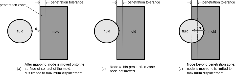
Penetration tolerance
This parameter is used to provide a tolerance level for the distance between the free surface and the mold surface. If a point on the free surface is located inside the mold at a distance from the mold surface below this tolerance, the point will not be moved; otherwise the position of the point is corrected. Three options are available: a value of 1 sets the penetration tolerance to be equivalent to the maximum displacement, by default, it is a fraction of the selected element size for the remeshing; a value of 2 sets the penetration tolerance to be equivalent to the minimum of the penetration accuracies; a value of 3 allows you to provide your own value for the tolerance, where it is recommended to keep the penetration tolerance to be less than or equal to the penetration accuracy.
The procedure for defining the mapping is as follows:
In the Global criteria for contact menu, select the Define mappings menu item.
Define mappings
The Mapping of free surfaces on molds menu will appear. You have the following options:
You can activate mapping contact boundary by contact boundary by selecting the Enable mapping along contact boundaries of mold [name of mold #i] menu item.
Enable mapping along contact boundaries of mold
[name of mold #i]
You can activate the mapping for all contact boundaries at once, by selecting the Enable Mapping along all contact boundaries menu item.
Enable Mapping along all contact
boundaries
You can disable the previous settings by selecting the following menu items:
Disable mapping along contact boundaries of mold
[name of mold #i]
or
Disable Mapping along all contact
boundaries
Select Numerical parameters for mapping/contact interpolation to modify the numerical parameters for all of the contact boundaries where the contact(s)/mapping(s) are defined.
Numerical parameters for mapping/contact
interpolation
To modify the threshold value allowing the mapping of a node, select the Modify threshold value = [current value] menu item.
Modify threshold value = [current
value]
To modify the scaling factor, select the Modify scaling factor = [current value] menu item.
Modify Scaling factor = [current value]
To modify the penetration tolerance, select the Modify penetration tolerance = [current value] menu item.
Modify penetration tolerance = [current
value]
To modify the maximum displacement, select the Modify maximum displacement = [current value] menu item.
Modify maximum displacement = [current
value]
To reset the default values, select the Reset to default values menu item.
Reset default values
To return to the Mapping of free surfaces on molds menu, select the Upper level menu menu item.
Upper level menu
If the flow sub-task contains planes of symmetry, they must be activated for the mapping. To do so, select the Planes of symmetry management menu item.
Planes of symmetry management
The Planes of symmetry management menu will appear, and Ansys Polydata will summarize the features and the status of each plane in the upper part of the panel. The status indicates whether the plane is activated, while the features provide information about its orientation. For the orientation, Ansys Polydata detects whether the plane is perpendicular to an axis of the coordinate system. The following is an example of the information displayed for a plane that is perpendicular to an axis:
Plane id 1 - plane perpendicular to X axis. -
                                    activated
The addition of
- activatedin the previous example indicates that the plane of symmetry has been activated for the mapping.The following is an example of the information displayed for a plane that is not perpendicular to an axis:
Plane id 2 - A=33, B=0.72, C=2.000001, D=
                                    0.01
You have the following options:
You can activate all of the planes of symmetry by selecting the Activate all planes (for mapping) menu item.
Activate all planes (for mapping)
You can activate individual planes of symmetry by selecting the Activate plane #i menu item.
Activate plane #i
You can deactivate all or single planes of symmetry by selecting the Deactivate all planes (for mapping) item or the Deactivate plane #i item, respectively.
Deactivate all planes (for mapping)
or
Deactivate plane #i
To correct the coefficient of the plane equation, select the Modify coefficients of a plane menu item.
Modify coefficients of a plane
When prompted, specify the plane index and the coefficient values.
For adaptive meshing for remeshing, Ansys Polyflow will refine elements
that have become too stretched and/or too distorted due to remeshing. An
element  will be refined if its quality is lower than the threshold
quality (
will be refined if its quality is lower than the threshold
quality ( ).
).
A quality value of 1 means that the element is not stretched or distorted
at all (for example, a square), and a value of 0 means that the element is
flat. The lower the value, the shape of the element will be more distorted.
All of the elements selected for refinement will be removed from the mesh,
and replaced by tetrahedra (in 3D) or triangles (in 2D) with the specified
size  .
.
For shell blow molding, since the recursive subdivision technique is used for refinement, an element selected for refinement because of its bad shape will be replaced by subelements with the same bad shape. Therefore, it is not useful to use adaptive meshing for remeshing in a shell blow molding simulation.
When you select Activate adaptive meshing for
remeshings, the Global criteria for
remeshings menu appears, where you can specify the values of
the parameters  and
and  (the size for new elements). The procedure for enabling
adaptive meshing for remeshing is the same as that for moving parts.
(the size for new elements). The procedure for enabling
adaptive meshing for remeshing is the same as that for moving parts.
To specify the values of the parameters, select the relevant menu items:
![]() Modify Tquality
Modify Tquality
![]() Modify Size
Modify Size
 is dimensionless, and its default is 0.8 for both 2D and
3D flows. The size
is dimensionless, and its default is 0.8 for both 2D and
3D flows. The size  has units of length, and its default value is the typical
size of segments in the mesh.
has units of length, and its default value is the typical
size of segments in the mesh.
It is important to note that the algorithm will pick up the elements that are picked for adaptive meshing, if at least one of the following conditions is met:
The quality is below the specified value of
 .
. The size is not within the interval
 .
.
Here, it is reasonable to select a size  that is compatible with the initial mesh. If you specify a
smaller value for the size
that is compatible with the initial mesh. If you specify a
smaller value for the size  , then elements satisfying the quality requirement will be
remeshed and refined in order to match the size criterion.
, then elements satisfying the quality requirement will be
remeshed and refined in order to match the size criterion.
In many applications involving large deformations of the mesh (glass pressing), the distortion mainly appears in some localized zones of the mesh. The features and details of the geometry that need small size for elements are also local in the mesh. The Manage zones for remeshing menu allows you to define very local regions where the size of the elements must be smaller to catch details of a geometry. The two types of zones available are: fixed zones and moving zones. The procedures for defining these zones are explained in the following sections.
- Boxes
Define the lower left corner and the upper right corner of the box.
- Circles/Spheres
Define the center and the diameter of the zone.
Click the Upper level menu when the dimensions of the zone are correctly defined.
Choose an appropriate element size for the zone, constant, or linear function of coordinates.
Note: The values used for the element size are very sensitive for the remeshing. It is recommended not to define an element size smaller than half the element size specified in the local criteria menu. If greater ratios are needed, a good solution is to define embedded zones with decreasing sizes to avoid badly shaped elements.
Click the Upper level menu when the element size of the zone is defined. The Manage zones for remeshing menu summarizes information about existing zones.
For glass pressing simulations, the peripheral material progressing along the molds is a critical region where the size cannot be too large. It is impossible to define a fixed zone because the periphery of the material is always moving. You could define a box that surrounds the whole flow region but this method demands the use of small elements over a large area and can lead to excessive CPU costs.
The Along boundaries zone option solves this problem. When you select this type of zone, you must specify the free surface on which you want to attach the moving zone. Choose the free surface and click the Upper level menu.
The parameters for the size are similar to those for adaptive meshing
parameters for contact. The size is calculated along the curvature of the
free surface using the (Equation 16–21). The parameters  and
and  have identical meaning. The parameter
  defines the depth of the zone.
You can define remeshing using the following procedure:
Define global or local criteria for adaptive meshing for remeshing.
Define
 for each subdomain (Local Criteria) or for all
subdomains (Global Criteria).
for each subdomain (Local Criteria) or for all
subdomains (Global Criteria). Define Size for each subdomain (Local Criteria) or for all subdomains (Global Criteria).
If there are contact problems, define global or local criteria for adaptive meshing for contact.
Define
 ,
,  , and
, and  for each contact problem (Local Criteria) or for all
contact problems (Global Criteria).
for each contact problem (Local Criteria) or for all
contact problems (Global Criteria). If some details need to be specified more accurately, define the zones.
If several sizes are defined simultaneously on an element through multiple criteria, the minimum of the size of all criteria encountered on this element is applied for the new size. It is important to understand that the criteria for adaptive meshing for contact and the zones for remeshing criteria only serve to define areas where size has to be smaller than that inside the subdomains. The element sizes specified in point 2 and 3 of the above procedure are smaller than that used in point 1.
The setup of adaptive meshing for remeshing (used, for example, for
pressing applications) involves two user parameters: the minimum element
size and the required element quality . The element size is a length which is defined as the
square root of the averaged edge squared lengths, and so, for example, the
element size of a regular tetrahedron with unit side lengths is one.
The quality is a global measure which invokes geometric features such as aspect ratio, angles between edges, and so on. Since adaptive meshing for remeshing only generates triangles and tetrahedra, respectively for 2D and 3D cases, focus will be applied to these two elements.
The of an equilateral triangle is one; if its height is
multiplied or divided by 2, the is 0.8. The of the standard right triangle is 0.86 and goes down to
0.4 when its height is four times larger or lower. This can be seen in Figure 16.21: Values for a Triangle Element vs Applied
Deformation where the
of these two suggested triangles is plotted versus the
height. Note that shearing the triangle also affects its .
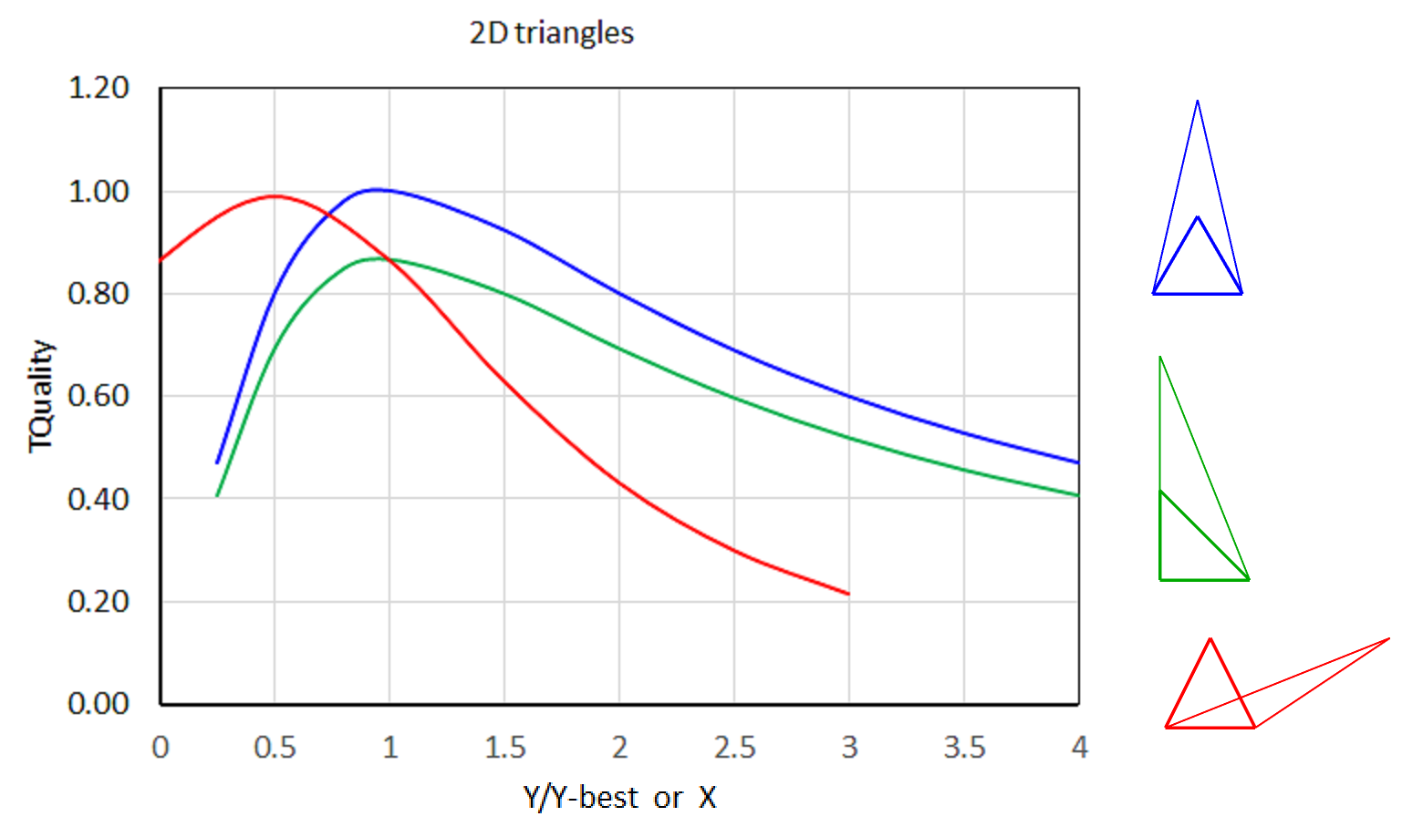
Note that the applied deformation is sketched on the right-hand side: vertical stretching of an initially equilateral triangle (blue), vertical stretching of an initially right isosceles triangle (green) and shearing of a triangle (red).
The description is a bit more complicated for a tetrahedron. The
of a regular tetrahedron is one; if its height is
multiplied by 3 or divided by 4, the is less than 0.45. The of the (standard) orthogonal tetrahedron is 0.77 and goes
down to less than 0.35 when its height is multiplied by 3 or divided by 4.
This can be seen in Figure 16.22: Values for a Tetrahedron Element vs Applied
Deformation
where the of these two suggested tetrahedra is plotted versus the
height. Note that shearing a tetrahedron also affects its . There are of course more degrees of freedom for deforming
a tetrahedron than a triangle, however they will not be explored here.
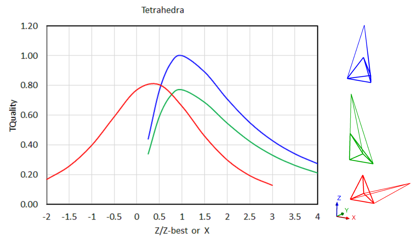
Note that the applied deformation is sketched on the right-hand side: vertical stretching of an initially regular tetrahedron (blue), vertical stretching of an initially orthogonal tetrahedron (green) and shearing of a tetrahedron (red).
When a Lagrangian remeshing is invoked for, for example, a pressing simulation, triangles in 2D and tetrahedra in 3D will always deform with the flow, it is reasonable to require a TQuality above what can be decently accepted, so that newly generated elements will still be endowed with enough quality after being deformed.