At the end of a shell blowing / thermoforming process simulation, Ansys Polyflow calculates the final thickness (and possibly temperature) distribution(s) through the blown / thermoformed product. It may also be useful to examine how the product cools and the deformations induced by such cooling. To do so, it is necessary to convert the shell mesh and result files into one of the following:
a full 3D mesh and corresponding result file.
a format that is suitable for a subsequent analysis with another software package. Currently, Ansys Polyflow can convert shell mesh and result files into a file that can be used as part of an LS-DYNA simulation.
Within the shell approximation for a multilayer system, the layer ordering is not relevant. Therefore, for such a multilayer system the thickness of a 3D mesh created from a shell mesh will be equal to the sum of all individual thicknesses.
The steps that follow describe how to convert shell meshes and result files.
For time-dependent or evolution problems, make sure that output files were saved at all of the time / evolution steps, intervals, or time values that are of interest to you. See Output for Time-Dependent, and Evolution Calculations for details.
Read the mesh file. If you did not use adaptive meshing, read the initial mesh file. If you used adaptive meshing for the shell blowing process, the last
adapt.mshfile generated by Ansys Polyflow (or a previous one, if relevant) should be read; note that in such a case, the files namedadapt.mshandrst.mshare the same.Click Convert shell mesh and results in the main menu of Ansys Polydata to open the Convert shell mesh and results menu.
 Convert shell mesh and results
Note that the format of the output files is not specified by default in the Convert shell mesh and results menu.
Specify the name of the Ansys Polyflow result file you would like to convert.
Enter the input result file name
Note that the result file should correspond with the mesh you read in step 2. Typically, you will specify the last
.resfile generated by Ansys Polyflow during the simulation of the shell blowing process. If you read a mesh file at a previous time step, however, you should specify the result file that was saved at that time step.Specify the domain to be extended into 3D.
Enter the shell domain
You have to select only the shell domain of your previous simulation. Be careful that you do not select the domains corresponding to the mold(s).
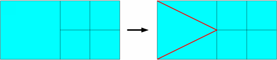
The next option concerns an optional refinement/unrefinement. By default, if adaptive meshing has been used in the previous simulation, a "conformalization" step will take place: elements adjacent to subdivided elements will be replaced in order to get a final mesh that is conformal (see Figure 7.14: Example of Conformalization):
However, it is also possible to restrain the levels of subdivision by specifying the minimum and maximum levels of refinement. To do so, select the Activate refinement/unrefinement menu item.
Activate refinement/unrefinement
When prompted, the Modify min and max levels of refinement item becomes available. Select this item:
Modify min and max levels of refinement
Then enter the desired range of refinement. All elements that have a level of refinement below the minimum will be refined, while those having a level higher than the maximum will be unrefined. If the minimum is not identical to the maximum level, a step of conformalization will be necessary and added automatically.
If you want to generate 3D mesh and result files, perform the following steps. Note that you can generate both 3D mesh and result files and an LS-DYNA output file at the same time.
Click the => Enable 3D mesh and result files generation menu item.
=> Enable 3D mesh and result files generation
Specify the mesh and result file names, by selecting the Enter the output mesh file name and the Enter the output result file name menu items, respectively. By default, the mesh and result files will be named
output.mshandoutput.res, respectively. With those files, it will be possible to define the simulation of cooling and thermoelastic deformations in another Ansys Polydata session.
Enter the output mesh file name
Enter the output result file name
Since it is possible to generate a 3D mesh by expansion of one side or the other side of the shell surface, you must specify the direction of generation. If you select the Specify direction of 3D generation menu item, the shell will be shown in the Graphics Display window with darts indicating the normal direction to the faces. By default, the mesh will be generated in that direction. A message appears also on your screen:
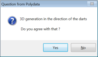
By selecting Yes or No, you can accept or change the direction of generation. Note that your selection appears in the comments of the menu:
3D generation in the direction of the darts
or
3D generation in the opposite direction to the darts
If the simulation contains plane(s) of symmetry, it is necessary to define them. To do so, select the Specify planes of symmetry menu item.
Specify planes of symmetry
A new menu will appear. By default, no constraints are applied on the directions of generation staying on boundaries of the shell domain. However, if planes of symmetry exist, the direction of generation must stay in such planes. To define such constraints, select each boundary B corresponding to a plane, then in the new menu Specify plane of symmetry along boundary B, switch to the Plane of symmetry option and enter the coefficients of the normal direction to the plane of symmetry.
Before running the conversion, you can check / modify some parameters used during the conversion. To do so, click the Advanced Options menu item.
Advanced Options
A new menu will appear that presents a set of numerical parameters. The most important parameter is the number of layers of elements. Three layers of elements are generated by default. By increasing the number of layers, you can better capture any thermal boundary layer. The distribution of elements in the thickness follows a Chebichef law.
Other parameters are needed by the iterative scheme used to generate a "good" 3D mesh. Indeed, the generated 3D elements may be distorted: too bended, too stretched, nonconvex, or with negative Jacobian, depending on the local curvature of the shell and the local thickness attached to that element. That is why you have to specify minimum angle, maximum angle, maximum bend and maximum skew. While all 3D elements do not respect those criteria, new small local deformations of the 3D mesh occurs to render the mesh well shaped. Note that the more stringent the criteria are, the more iterations are needed (and a solution may not be found that respects that criteria). As a side effect of this procedure, the boundaries of the 3D mesh that are adjacent to the shell surface will probably not remain perpendicular to the shell surface.
In order to facilitate the generation of well shaped 3D elements, all quadrilateral faces of the shell surface that are too bended or that have a high internal angle will be divided into two triangles. The parameters that fix the limit are maximum bend for faces and maximum angle for faces, respectively.
For any 3D element, if its starting face does not respect the criteria mentioned previously, then the criteria applied on the element will be based on the limits of the starting face multiplied by (1+tolerance) or (1-tolerance). For example, if a given starting face has a minimum angle between two segments equal to
 and the minimum angle specified is
  , then the minimum angle that will effectively be
applied for the criteria is
, then the minimum angle that will effectively be
applied for the criteria is  . Note that the small deformations applied on the 3D
mesh are based on the local reorientation of the direction of
generation. The starting shell surface is never deformed.
. Note that the small deformations applied on the 3D
mesh are based on the local reorientation of the direction of
generation. The starting shell surface is never deformed. Another parameter that affects the speed of convergence of the iterative scheme is the mode of update of the local normals to the shell surface. The delayed mode seems to be faster than the immediate mode. The default value (delayed mode) should not be modified.
For debugging purpose, it is possible to write in the listing file more information by changing the verbosity (from minimum to maximum).
To accept the values of the numerical parameters, click the Upper level menu menu item.
Upper level menu
You will return to the Convert shell mesh and results menu.
If you want to generate an LS-DYNA output file, perform the following steps. Note that you can generate both an LS-DYNA output file and 3D mesh and result files at the same time.
Click the => Enable LS-DYNA output generation menu item.
=>Enable LS-DYNA output generation
Specify the name for the LS-DYNA output file, by clicking the Enter the output LS-DYNA file name menu item and entering the name in the dialog box that opens. By default, the output file will be named
output.dyn. You will use this file to define a simulation in LS-DYNA.
Enter the output LS-DYNA file name
Click the Convert and exit or the Save and exit menu item to run an Ansys Polyflow simulation that generates the 3D mesh and result files and/or LS-DYNA output file. The following message will appear to verify that you want to run the calculation:
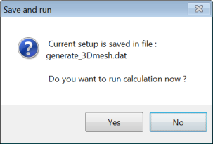
By clicking Yes, you will run Ansys Polyflow immediately. In any case, a data file is generated (
generate_3Dmesh.dat) for further use.A listing file will be produced by Ansys Polyflow, which provides information about the steps of the convergence (for example, the number of distorted 3D elements decreasing with the number of iterations, information about the mesh conformalization, interpolation of thickness fields, and so on). The following is an example of the listing file produced when generating 3D mesh and result files.
 ****************************
 *                          *
 * Shell to 3D conversion   *
 *                          *
 ****************************

 Shell ...................... : shell support
 Thickness field(s) ......... : THICKNESS
 Isothermal shell
 3D generation along the normal to the faces
 Number of layers of elements :   3
 Maximum number of iterations : 500
 Update of normals .......... : delayed mode
 Information printed ........ : min.
 Minimum interior angle ..... : 0.2000000E+02
 Maximum interior angle ..... : 0.1600000E+03
 Maximum bend ............... : 0.8000000E+00
 Maximum skew ............... : 0.1000000E+02
 Maximum angle for faces .... : 0.1600000E+03
 Maximum bend for faces ..... : 0.1000000E+00
 Tolerance .................. : 0.1000000E+00

 + Planes of Symmetry

 Plane (S1*B3).
 of normal direction : 0.1000000E+01 0.0000000E+00 0.0000000E+00

 Iteration 1, # distorted elements = 795 / 18536
 Iteration 2, # distorted elements = 552 / 18536
 Iteration 3, # distorted elements = 565 / 18536
 Iteration 4, # distorted elements = 511 / 18536
 Iteration 5, # distorted elements = 485 / 18536
 ...
 Iteration 251, # distorted elements = 4 / 18536
 Iteration 252, # distorted elements = 3 / 18536
 Iteration 253, # distorted elements = 2 / 18536
 Iteration 254, # distorted elements = 1 / 18536
 Iteration 255, # distorted elements = 0 / 18536

 Quality of 3D elements : final check

>>  Number of distorted elements = 0 / 18536
Note: The divisor displayed for the number of distorted elements for each iteration (
18536in the previous example) represents the number of starting faces (after all possible faces have been divided into triangles).