


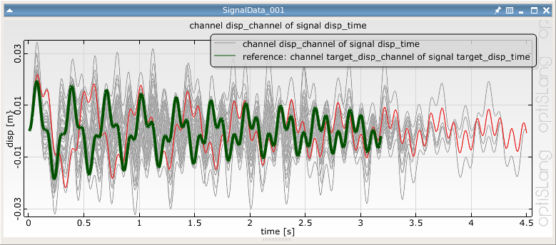
If signal data is available, you can visualize it using this plot. You can choose the signal data to visualize (colored grey) using the settings in the Common settings pane. You can also plot a reference signal by selecting from the available signal data and specifying a signal, a channel and a design. Since each successfully calculated design corresponds with one curve of the plotted array of curves, this plot provides the same features of design selection, activation and coloring as other plots. Curves belonging to selected designs are colored red.
Signal MOP
If Signal MOP data is available, you can select the Signal MOP results from the list of available signals. For each signal, two additional signals with the suffixes _SoS and _Variability_fractions are added. The individual results are:
F-CoP (%)
This shows the prognosis quality (F-CoP[Total]) and sensitivity indices (F-CoP[input]) of the field meta model for the respective signal as a relative value (percentage).
The prognosis quality is a value between 0 and 100% (as is CoP for MOP). It may be a different value for individual regions on the abscissa. This means that the Signal MOP may represent the original process well in some regions while it represents the original process not so well in other locations on the abscissa. You should also compare it with the amount of variation (for example, the standard deviation): Typically the prognosis quality is not well for regions with small variations. This can, however, often be neglected since it is necessary to represent large variations accurately, but not near-deterministic values.
The sensitivity indices define how sensitive the signal is changing with respect to changes of the individual parameters. This sensitivity may also be different for individual locations on the abscissa. E.g. for a load-displacement curve in structural mechanics, the elastic modulus will typically be dominant for small strains while damage parameters will be more important for larger strains.
F-CoP (abs.)
This shows the prognosis quality (F-CoP[Total]) and sensitivity indices (F-CoP[input]) of the field meta model for the respective signal in the unit of the original signal. This is achieved by multiplying the square root of the F-CoP (R^2) with the actual standard deviation of the signal. The resulting quantity is called R*sigma.
The Rsigma plot illustrates the prognosis quality and sensitivity indices with respect to the actual amount of variation. Comparing Rsigma[Total] with the true standard deviation sigma, you can estimate the amount of variation which can be represented by the meta model at each respective location. In a similar way, the single Rsigma curves indicates what amount of variation of the signal is contributed by a single input.
Correlation
This plot shows the correlation coefficient between the signal and the individual input parameters. This is equivalent to a single row in the optiSLang correlation matrix associating a single response the input parameters.
While the F-CoP defines the sensitivity based on nonlinear relations, the correlation defines the sensitivity based on an assumed linear relationship. It can further be negative with values between -1 (100% negative correlation) and 1 (100% positive correlation).
Signal statistics
This plot shows some statistical data of the analysed signal sample. It shows:
Minimum and Maximum as the absolute lower and upper bounds of all signals found in the sample.
Lower and Upper 5% quantile values.
Lower and Upper 25% quantile values.
Mean signal.
Median signal (50% quantile value).
Scatter shapes
This plot shows the variation patterns (scatter shapes) that were identified. Only as many scatter shapes are shown which are necessary to create the empirical random field model.
Each variation pattern represents a single mechanism acting in the observations of the signals. The scatter shapes are ordered according to their statistical importance.
Each signal can be represented by a linear combination where each variation pattern is scaled by some (positive or negative) number and added to the mean value signal. The individual scatter shapes are associated with statistically uncorrelated scaling factors. The scaling factors are called random field amplitudes. Their properties and individual metamodels can be monitored by a separate OMDB file, if was selected in the Signal MOP settings.
Variability fractions
This plot shows the distribution of the variability fraction associated with each scatter shape. The variability fraction is the portion of the signal variance that can be explained by each individual scatter shape. Displayed values are averages over the entire abscissa.
The individual variability fraction is computed for each scatter shape. The cumulative variability fraction indicates the amount of explainable variance obtained when taking as many scatter shapes. If, for example, the cumulative variability fraction for abscissa value 6 is 90.5%, then you require at least six shapes to represent 90.5% of signal variance as compared to the sample data.
The variability fraction plot also gives hints on the correlation of the signal along the abscissa. If few (for example, less than five) scatter shapes suffice to represent a large variability fraction (for example, 90%), then the signal is strongly correlated. Vice versa, if many shapes (for example, more than ten) are needed, the signal is weakly correlated, maybe noisy.
Settings
| Option | Description |
|---|---|
| Common Settings | |
| Signal | Select the signal data to display. |
| Channel | Select the channel data to display. |
| Reference signal | Select the reference signal data to display. |
| Reference channel | Select the reference channel data to display. |
| Adjust resolution | When selected, displays the Resolution and Interpolation type settings. |
| Resolution | Adjusts the resolution with the given interpolation type for all viewed signal lines. |
| Interpolation type | |
| Show statistical value | When selected, displays the Sigma factor setting. |
| Sigma factor | Displays mean and sigma lines with the given sigma factor for the signal set with the Signal and Channel settings. |
| Show as contour plot | When selected, displays the Number of classes, Palette minimum value, and Palette maximum value settings. |
| Number of classes | Select the number of classes for the colored plot. |
| Palette minimum value | Sets the minimum value of the palette for the colored plot. |
| Palette maximum value | Sets the maximum value of the palette for the colored plot. |
| Preferences | |
|
The following preference settings are available:
For more details, see Plot Preference Settings. | |
Python Scripting
Create Visual
Creates a signal plot using data with data_id.
signal_plot = Visuals.SignalPlot(Id("Signal plot"), data_id)
Add to Postprocessing
Adds signal plot in postprocessing to control_container, using the specified relative positioning.
    control_container.add_control (
        signal_plot,
        True,
        RELATIVE_POSITIONING,
        0., 0., 1., 1./2.
    )