Deep infinite mixture of Gaussian processes (DIM-GP) is a unique combination of neural networks and Gaussian processes that combines the advantages of both modeling techniques, overcoming many disadvantages of each one. It is suitable for a variety of machine learning applications such as regression and classification for scalar quantities. DIM-GP is also suitable for any number of samples as well as any number of input parameters. The number of samples loaded into memory at one time can be controlled by setting the batch size. At very high sample numbers the prediction time may slow down depending on the batch size setting. DIM-GP is also suitable for noisy data, since an additional noise parameter is trained internally. This can also be used to automatically avoid outliers, for example. Detailed information about the algorithm can be found here.
Usage
DIM-GP for Signal Data modeling is an enhancement for the MOP, allowing you to model signal-type data. It supports x-y-data as well as signal response types.
The DIM-GP Signal model must be activated explicitly using the MOP node advanced settings. It can only be activated if either of the supported response types is declared on the list of responses.
Once the model type is activated in the MOP settings, running the MOP node starts the DIM-GP model training. This trains an analytical model that maps the scalar input parameters to the selected signal type responses. Information about the quality of the trained model can be investigated using the optiSLang postprocessing, by studying the CoP curve using the signal plot. Given a trained DIM-GP signal model, the MOP Solver node can be used to serve the model and use it in an approximation context.
Advanced Settings
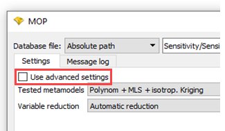
You can access the DIM-GP Signal advanced settings in the MOP settings dialog box.
Right-click the MOP node and select from the context menu.
Select the Use advanced settings check box.
In the Advanced Settings tab, under DIM-GP Signal, select the Use check box.
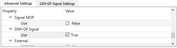
Switch to the DIM-GP Signal Settings tab.
Change the settings as required.
Name Default value Description Maximum epochs 1000 Maximum number of training epochs used. Algorithm messages provide hints for the required number of epochs.
Batch size 0 (disabled) Batch training can reduce computational costs for the training of the neural network model. Batch training is activated if the defined Batch size is non-zero and smaller than the overall number of training samples. Using this option is recommended for large number of training data sets.
Noisy data Off (disabled) Enable the Noisy data setting if any type of noise is expected in the training dataset. The training procedure will be configured for a stronger smoothing on the output side. DIM-GP Advanced Settings Off Activates or deactivates the advanced settings for this model. Job Submit Pattern (beta) <jobscript> <arg1> <arg2> <arg3> Specifies the job submit pattern for bash or command prompt for submitting jobs. Will be cast with
subprocess.popen. First argument<arg1>is for submitting jobs, the second argument<arg2>is for defining a submission pattern that allows a list of arguments to be passed to the job. The third argument<arg3>is for defining the directory.If the last entry does not exist, the action will be skipped and if empty, arguments will be submitted without an optional argument command.
Output Compression Method PCA Method to reduce the dimensionality of the outputs. The options are:
GAE (Gated Recurrent Units auto-encoder)—Beta
AE (auto-encoder)—Beta
KPCA (kernel PCA)—Beta
PCA (principle component analysis)—Default
Note: AE and GAE may take longer to run as optiSLang must train a neural network to reduce the output dimensionality.
Apply Signal Transformation Off (disabled) If this setting is enabled, a power transformation is applied to the signal responses in a pre-processing step before the actual model training. The response data is transformed to distribute the output data uniformly and stabilize the variance. Such transformation can be beneficial for the model training. Channel Cross-Correlation On (enabled) Specifies whether treating channels of signals of multiple channels as cross-correlated, by means of the model can exploit interdependencies between the channels of a signal response. In case of independent channels, disabling this option is expected to improve the prognosis quality. For each channel an independent model is build, which comes at higher computational costs. To save and close the dialog, click .
Output Compression Methods
- Principle Component Analysis (PCA)
Decomposes the signals of linearly dependent signal steps into non-correlated principal components. Instead of the signal steps themselves, the principal components are then used as output in the model. In the prediction, the model prediction representing the principal components is then transformed back to the original signal steps. In contrast to the auto-encoder based compression methods (GAE, AE), PCA belongs to the deterministic methods. For the same input, the same compression of the output data takes place, and the same principal components are created. This method should be used if the signal time steps are mostly linearly correlated.
- Kernel Principle Component Analysis (KPCA)
Works in principle in the same way as PCA. The only difference is that by applying non-linear kernel functions to the signal data, that then also non-linearly correlated data can be decomposed into principal components. This method can therefore be advantageous if the signal steps are highly non-linear correlated.
- Auto-Encoder (AE)
Compression method based on neural networks. The dimensionality of the signal steps is reduced by a so-called encoder part in which the number of neurons in the layers is reduced step by step. These encoded substitute dimensions are then used as output instead of the original signal steps in the model training. Another decoder part is needed to bring the encoded substitute dimensions back into the original space. This is another network in which the number of neurons increases again step by step in the levels until the original number of signal steps is restored. The auto-encoder is trained so that the difference between input data and predicted data in the decoder part is as small as possible. This type of compression method is also suitable for uncorrelated signal steps similar to KPCA, but is even more flexible since no kernel function is fixed.
- Gru Auto Encoder (GAE)
Works like AE except that instead of normal feed forward layers, so-called GRU layers are used. These layers can learn time dependencies in the signal steps similar to recursive networks. It learns explicitly the behavior of the x previous signal steps which are not explicitly considered in the other compression methods. This compression method can be especially useful if the signal data has recurring patterns, for example the behavior of previous steps leads to a certain behavior of subsequent steps.
Note that Auto-Encoder based compression methods (AE / GAE) take more time compared to (PCA / KPCA) since a neural network must be trained. So the overall training of the signal model might take longer. Non-linear compression method might some time lead to non-smooth model predictions. If this is a problem you should try to use PCA instead.
External Files
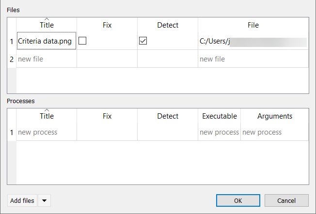
DIM-GP Signal makes use of external files that store the model and meta information. The location of those files is stored in the optiSLang postprocessing file (*.omdb). These file locations can be viewed and edited, if necessary. To do so:
Open the *.omdb file by selecting > from the menu bar.
Open the Manage files and processes dialog box by selecting > from the menu bar.