


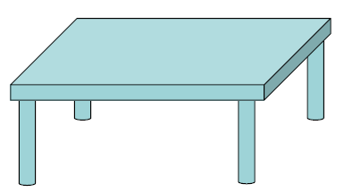
This tutorial allows you to build an application to design a table.
To build this application:
Gather the customer inputs
Required size
Load
Maximum cost
Calculate costs
Prove the design using simulation
Store the design
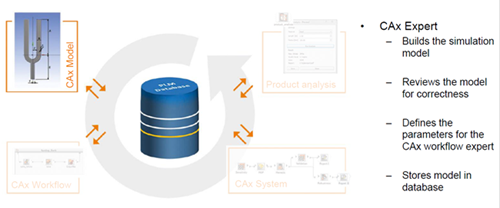
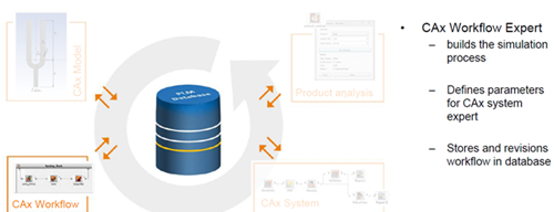
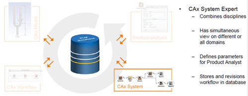
CAx Experts:
Python expert: Create Table top model
MATLAB expert: Create Table leg model
Excel expert: Create Table cost model
optiSLang expert: Create Table load model
Simulation expert: Create sub-optiSLang Table load project.
Workflow expert:
Combine simulation models
Calculate total table cost and table load if the total cost is less than the maximum cost
Add load simulation
Publish workflow
User (manager or a customer): Run and use the workflow.
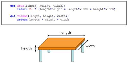
Python Expert
Calculate volume and area of the table top using Python.
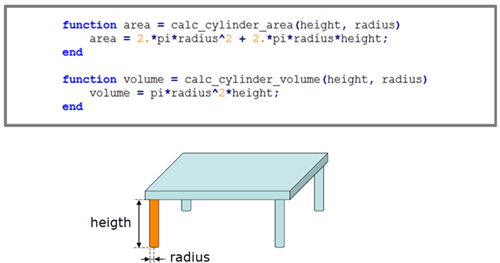
MATLAB Expert
Calculate volume and area of one table leg using MATLAB.
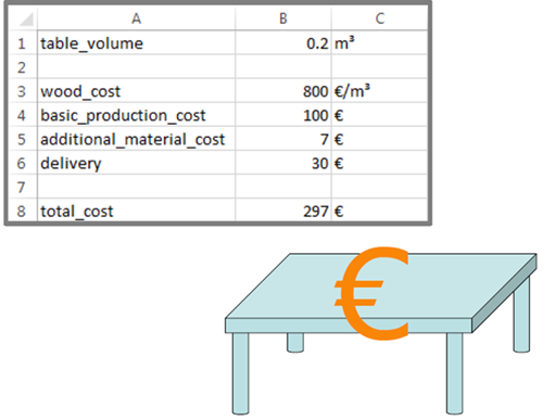
Excel Expert
Calculate table costs using Excel.
optiSLang Expert
Calculate table stress level using optiSLang.
Simulation Expert
Create the Table load optiSLang project. For more details, see Creating the Table Load Model using optiSLang.
Workflow Expert
Creates and publishes the workflow. For more details, seeCreating the Table Workflow and Publishing the Workflow.

You must install the optiSLang Web Service (web interface for optiSLang) before starting this tutorial.
Before you start the tutorial, download the table zip file from here , and extract it to your working directory.
In this section of the tutorial, you will:
Generate a solver chain using text based optiSLang solver
Define the parameters and responses
Define the solver call setup
Specify parameter properties
To complete this section of the tutorial, perform the following steps:
- Creating a New Table Load Project
- Selecting the Input File
- Defining the Input Parameters
- Editing the Parameter Properties
- Selecting the Output File
- Defining the Response
- Adding a New Variable
- Defining the Optimization Criteria
- Importing the Solver Call File
- Finishing the Solver Wizard
- Saving and Running the Table Load Project
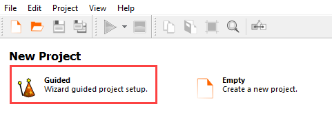
Start optiSLang.
Create a new guided project.
Expand .
Clear the Create in parametric system check box.
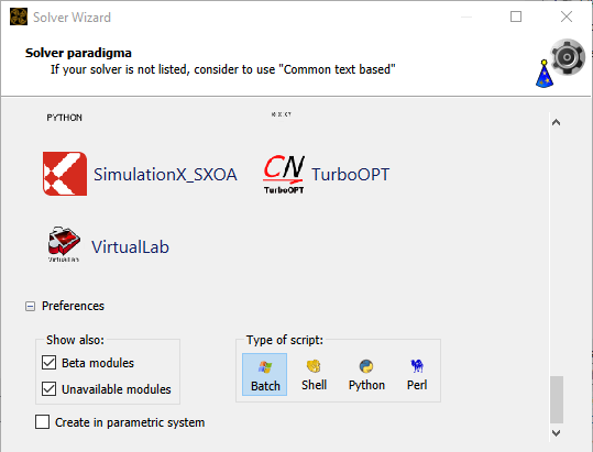
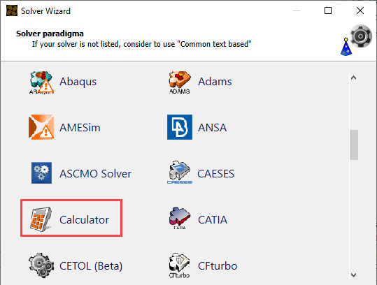
From the solver list, click .
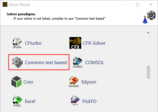
In the Select input file dialog box, browse to the table folder and select table.s.
Click .
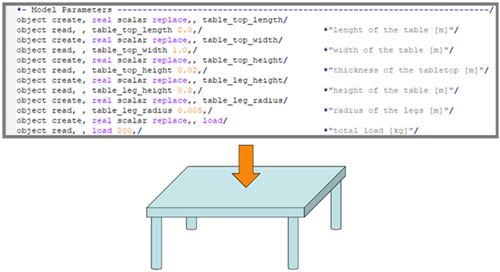
In the text editor, highlight
object read, ,
                            table_top_length
.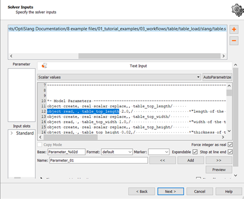
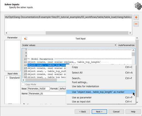
Right-click the selection and select from the context menu.
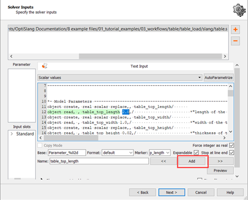
Highlight the number to the right of
object read, , table_top_length.Rename the parameter to
table_top_length.To register the parameter, click Add.
Repeat this procedure for
table_top_width, table_top_height,
                            table_leg_height, table_leg_radius, load
.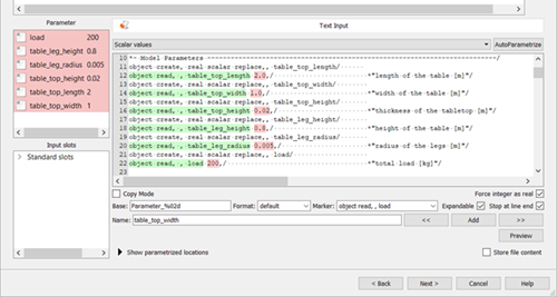
Click .
Double-click the range numbers for row 1 (table_top_length).
Change the lower bound to
0.8and the upper bound to1.2.Double-click the range numbers for row 2 (table_top_width).
Change the lower bound to
1and the upper bound to5.Double-click the range numbers for row 3 (table_top_height).
Change the lower bound to
0.01and the upper bound to0.07.Double-click the range numbers for row 4 (table_leg_height).
Change the lower bound to
0.7and the upper bound to0.9.Double-click the range numbers for row 5 (table_leg_radius).
Change the lower bound to
0.01and the upper bound to0.02.Double-click the range numbers for row 6 (load).
Change the lower bound to
0and the upper bound to500.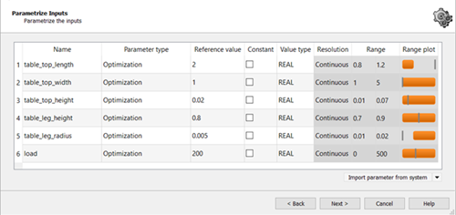
Click .
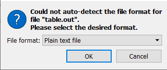
In the Choose a file to open dialog box, browse to the table folder and select table.out.
Click .
From the File format list, ensure is selected and click .
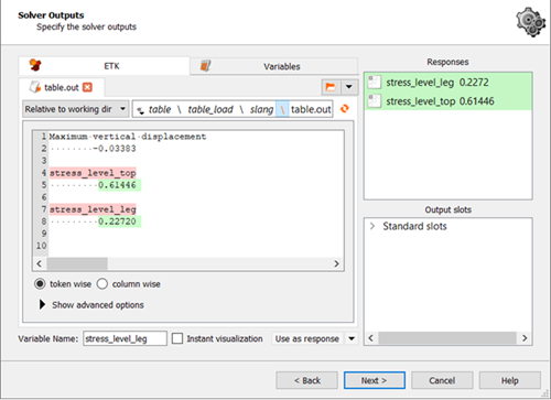
Highlight the text in line 4 (stress_level_top).
Right-click the selection and select > from the context menu.

Click .
Repeat steps 2-4 with stress_level_leg.
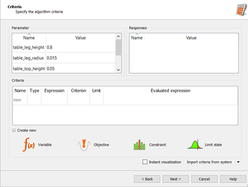
Switch to the tab.
Click .
Click the ID cell of the new variable, type
load_proofedand press Enter.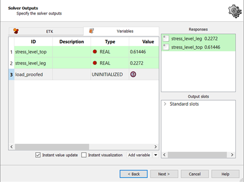
Right-click the Expression cell of row 3 (load_proofed) and select from the context menu.
Enter the following conditional expression:
#IF (stress_level_leg<= 1.0)&& (stress_level_top<= 1.0) #THEN 1#ELSE 0
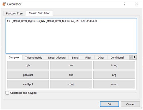
Click .
Drag the load_proofed row into the Responses pane to register it as a response.
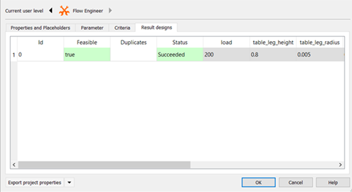
Click .
Do not adjust or add to the currently displayed values for parameters, responses, and criteria.
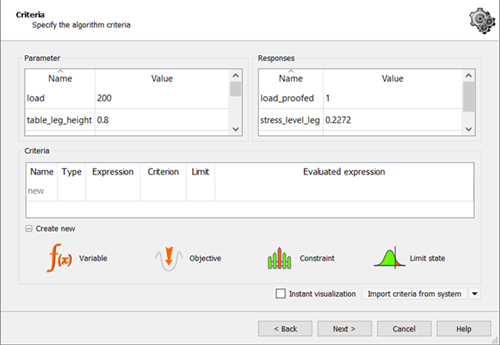
Click .
To the right of the Absolute path field, click the orange folder.
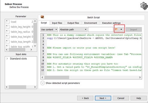
Browse to the table folder and select table.bat for Windows systems or table.sh for Linux systems.
Click .
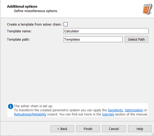
Click .
Ensure the Create a template from solver chain check box is clear.

Click .
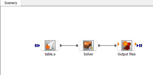
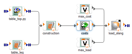
The solver chain is displayed in the Scenery pane.
In this section of the tutorial, you will:
Generate a solver chain
Define the parameters and responses
Use conditional execution
To complete this section of the tutorial, perform the following steps:
- Creating a New Table Workflow Project
- Selecting the Table Top Input File
- Selecting the Table Top Parameters and Outputs
- Editing the Table Top Parameter Properties
- Defining the Table Top Optimization Criteria
- Finishing the Table Top Solver Wizard
- Starting the Table Leg Solver Wizard
- Selecting the Table Leg Parameters and Outputs
- Editing the Table Leg Parameter Properties
- Defining the Table Leg Optimization Criteria
- Finishing the Table Leg Solver Wizard
- Creating the Construction Node
- Saving and Running the First Part of the Table Workflow Project
- Creating the Table Costs Node
- Saving and Running the Second Part of the Table Workflow Project
- Creating the Variable Nodes
- Creating the optiSLang Node
- Saving and Running the Third Part of the Table Workflow Project
Start optiSLang.
From the Start screen, click .
Expand .
Clear the Create in parametric system check box.
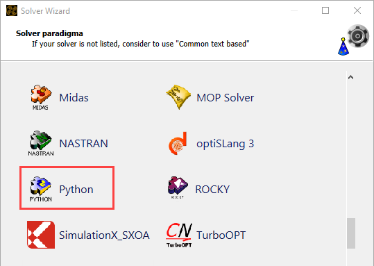
From the solver list, click .
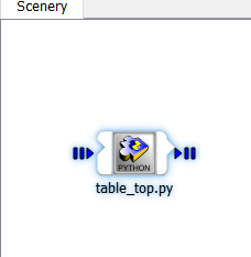
In the Select input file dialog box, browse to the table folder and select table_top.py.
Click .
From the Detect assignments drop-down list, select .
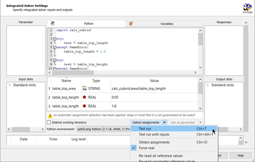
In the Python table, select table_top_height, table_top_length and table_top_width and drag them to the Parameter pane.
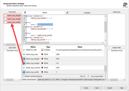
In the Python table, select table_top_area and table_top_volume and drag them to the Output slots pane.

Click .
Double-click the range numbers for row 1 (table_top_height).
Change the lower bound to
0.01and the upper bound to0.07.Double-click the range numbers for row 2 (table_top_length).
Change the lower bound to
1and the upper bound to5.Double-click the range numbers for row 3 (table_top_width).
Change the lower bound to
0.8and the upper bound to1.2.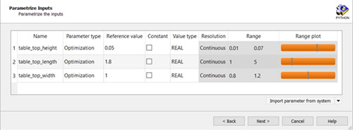
Click .
Do not adjust or add to the currently displayed values for parameters, responses, and criteria.
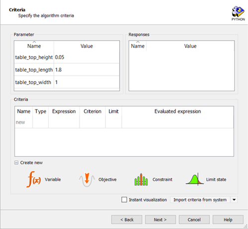
Click .
Ensure the Create a template from solver chain check box is clear.
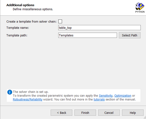
Click .
The solver chain is displayed in the Scenery pane.
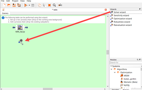
From the Wizards pane, drag the Solver wizard to the Scenery pane and let it drop.
Expand .
Clear the Create in parametric system check box.
From the solver list, click .
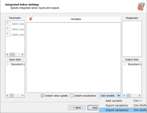
From the Add variable drop-down list, select .
In the Open optiSLang variables from file dialog box, browse to the table folder and select table_leg.ovdb.
Click .
In the Variables table, select all rows and drag them to the Parameter pane.
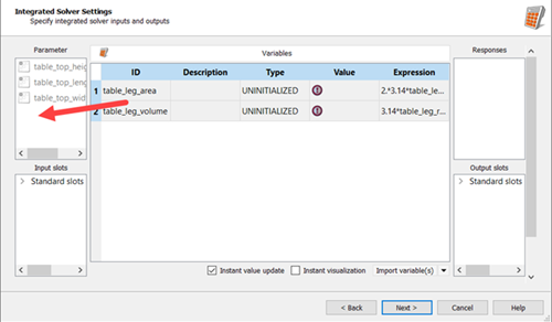
In the Value field for table_leg_height enter
0.8and click .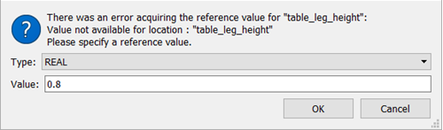
In the Value field for table_leg_radius enter
0.015and click .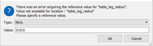
In the Variables table, select all rows and drag them to the Output slots pane.
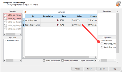
Click .
Double-click the range numbers for row 4 (table_leg_height).
Change the lower bound to
0.7and the upper bound to0.9.Double-click the range numbers for row 5 (table_leg_radius).
Change the lower bound to
0.01and the upper bound to0.02.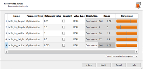
Click .
Do not adjust or add to the currently displayed values for parameters, responses, and criteria.
Click .
Ensure the Create a template from solver chain check box is clear.
Click .
Right-click the Calculator node and select from the context menu.
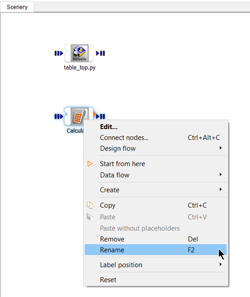
Type
table_legand press Enter.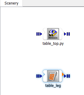
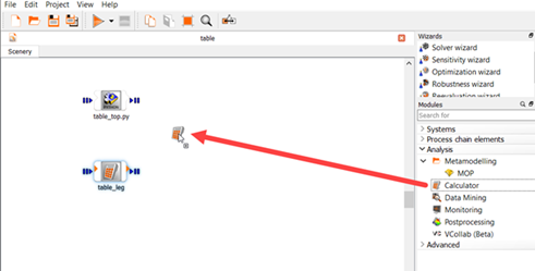
Under Modules, expand .
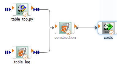
Drag a Calculator node onto the Scenery pane and let it drop.
Right-click the Calculator node and select from the context menu.
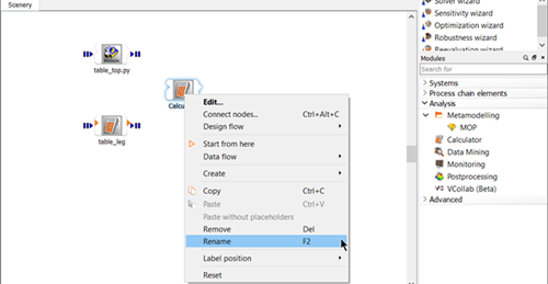
Type
constructionand press Enter.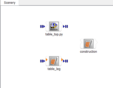
From the menu bar select > > .
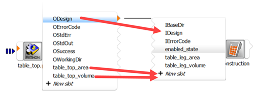
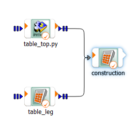
Hover over the right side of the table_top node.
Make the following connections by clicking the items on the table_top node list and dragging them onto the list on the left side of the construction node.
ODesign to IDesign
table_top_area to New slot
table_top_volume to New slot
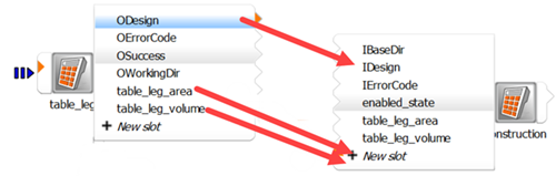
Hover over the right side of the table_leg node.
Make the following connections by clicking the items on the table_leg node list and dragging them onto the list on the left side of the construction node.
ODesign to IDesign
table_leg_area to New slot
table_leg_volume to New slot
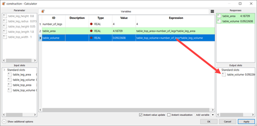
Double-click the construction node.
To add three new variables, click three times.
Double-click the ID cell for variable_1, type
number_of_legs, and press Enter.Double-click the Expression cell, type
4, and press Enter.Double-click the ID cell for variable_2, type
table_area, and press Enter.Double-click the Expression cell, type
table_top_area+number_of_legs*table_leg_area, and press Enter.Double-click the ID cell for variable_3, type
table_volume, and press Enter.Double-click the Expression cell, type
table_top_volume+number_of_legs*table_leg_volume, and press Enter.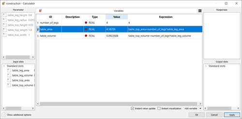
In the Variables table, select rows 2 and 3 (table_area and table_volume) and drag them to the Responses pane.
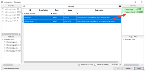
In the Variables table, select row 3 (table_volume) and drag tit to the Output slots pane.
Click .
To save the project, click
 .
.Browse to the location to save the project and type
tablein the File name field.Click .
To run the project, click
 .
.Check that all nodes have executed successfully.
Under Modules, expand and .
Drag an Excel node onto the Scenery pane and let it drop.
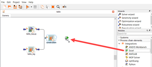
Right-click the Excel node and select from the context menu.

Type
costsand press Enter.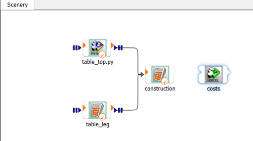
Double-click the costs node.
To the right of the Absolute path field, click the orange folder.
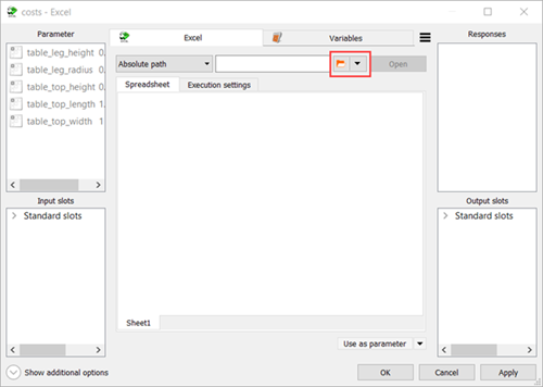
In the Choose a file to open dialog box, browse to the table folder and select table_cost.xlsx.
Click .
In the Excel table, select row 1 (table_volume) and drag it to the Input slots pane.
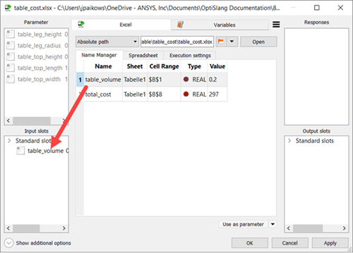
In the Excel table, select row 2 (total_cost) and drag it to the Responses and Output slots panes.
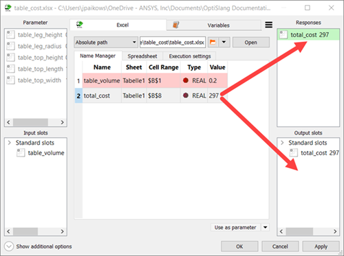
Click .
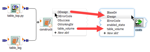
Hover over the right side of the construction node.
Make the following connections by clicking the items on the construction node list and dragging them onto the list on the left side of the costs node.
ODesign to IDesign
table_volume to table_volume
To save the project, click
.To run the project, click
.Check that all nodes have executed successfully.
Under Modules, expand and .
Drag two Variable nodes onto the Scenery pane.
Right-click the Variable node and select from the context menu.
Type
max_costand press Enter.Right-click the Variable (1) node and select from the context menu.
Type
max_loadand press Enter.
Double-click the max_cost node.
From the data kind list, select .
Double-click the row 1 cell.
Type
300and press Enter.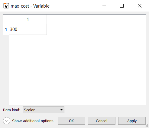
Click .
Double-click the max_load node.
From the data kind list, select .
Double-click the row 1 cell.
Type
50and press Enter.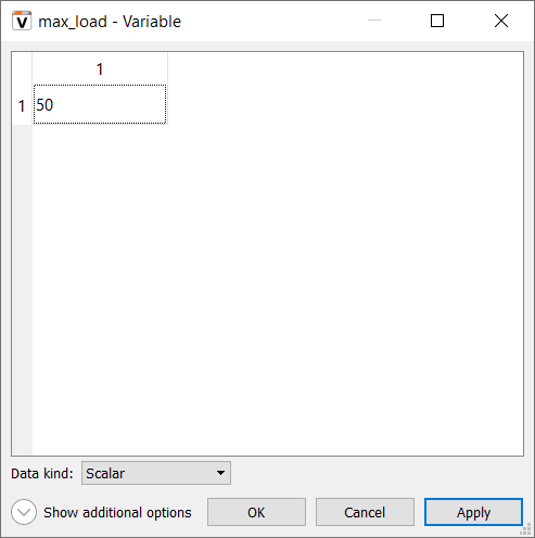
Click .
Under Modules, expand and .
Drag an optiSLang node onto the Scenery pane and let it drop.
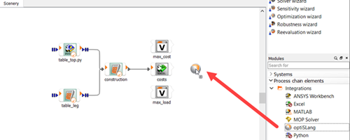
Right-click the optiSLang node and select from the context menu.
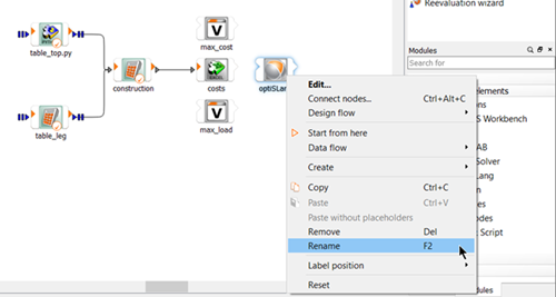
Type
load_slangand press Enter.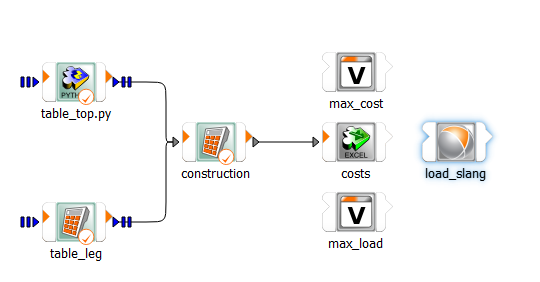
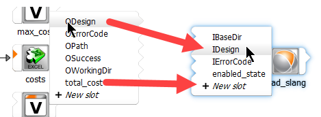
Hover over the right side of the costs node.
Make the following connections by clicking the items on the costs node list and dragging them onto the list on the left side of the load_slang node.
ODesign to IDesign
total_cost to New slot
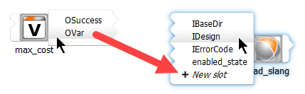
Hover over the right side of the max_cost node.
Click OVar and drag tit onto the list onto the New slot on the left side of the load_slang node.
Hover over the left side of the load_slang node.
Right-click the OVar input slot and select from the context menu.
Type
max_costsand press Enter.Double-click the load_slang node.
To the right of the Absolute path field, click the orange folder.
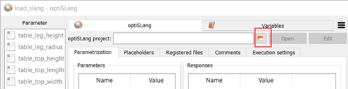
In the Choose a file to open dialog box, browse to the location where you saved the table_load_slang project and select table_load_slang.opf.
Click .
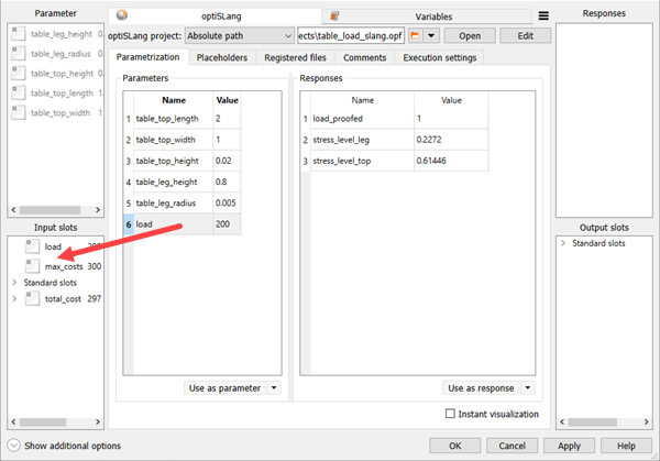
In the Parameters table, select row 6 (load) and drag it to the Input slots pane.
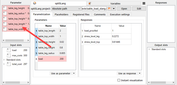
In the Parameters table, select rows 1-5 and drag them to the Parameter pane.
In the Responses table, select rows 1 (load_proofed) and drag it to the Responses pane.
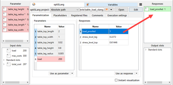
Click
 .
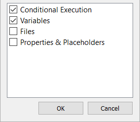
.Select the Conditional Execution check box.
Click .
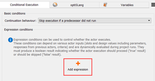
Switch to the Conditional Execution tab.
From the Continuation behaviour list, select .
Click Add expression.
In the Expression field type
total_cost<max_costand press Enter.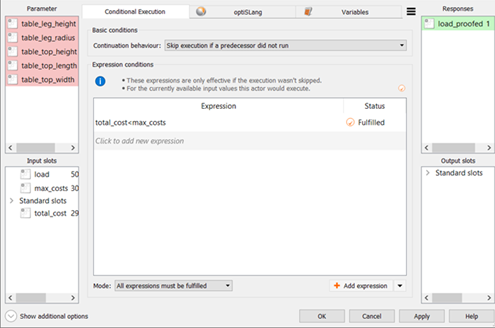
Click .
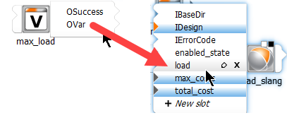
Hover over the right side of the max_load node.
Click OVar and drag tit onto the list onto the load input slot on the left side of the load_slang node.
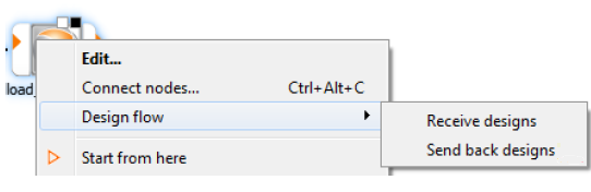
Right-click the load_slang node and select > .
In this section of the tutorial, you will:
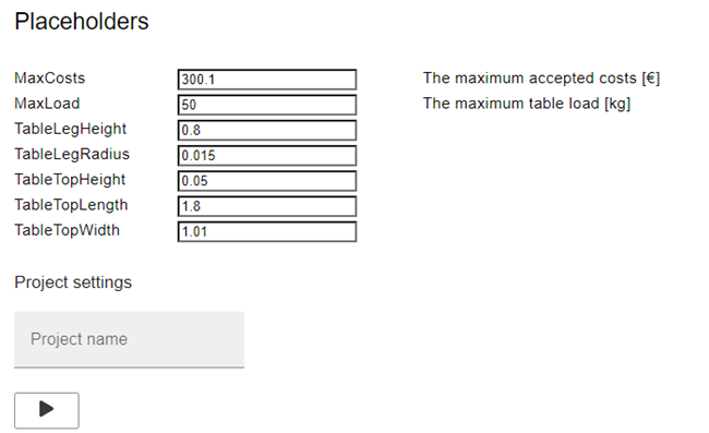
Define the project placeholders
Publish the workflow
To complete this section of the tutorial, perform the following steps:
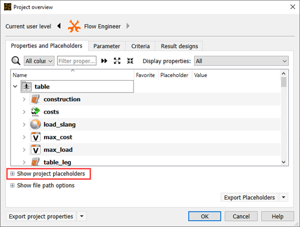
With the table.opf project open, select > from the menu bar.
Expand Show project placeholders.
In the Filter properties field, type
Variant.Under max_cost, drag Variant onto new placeholder.
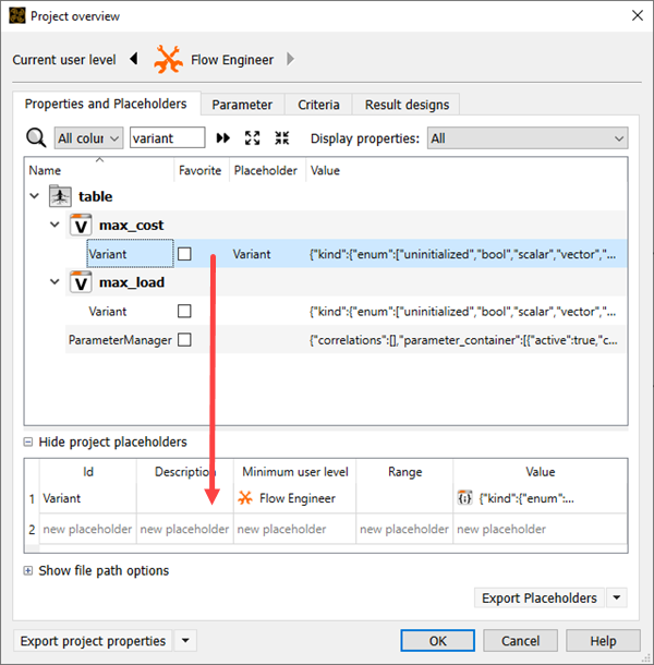
Click the Id cell for row 1 and change the name to
MaxCostVariant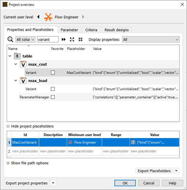
Under max_load, drag Variant onto new placeholder.
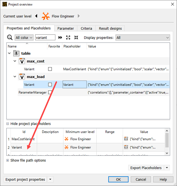
Click the Id cell for row 2 and change the name to
MaxLoadVariant.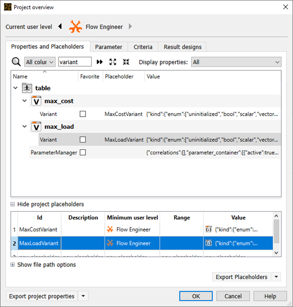
In the Filter properties field, type
parameter.Under table, drag ParameterManager onto new placeholder.
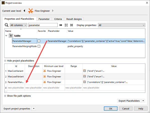
In the Id cell of the new placeholder row, type
TableTopHeight.Double-click the Minimum user level cell and select from the list.
In the Range cell, type
[0.01-0.07].Double-click the Value cell and select from the list.
In the Expression field, type
0.05.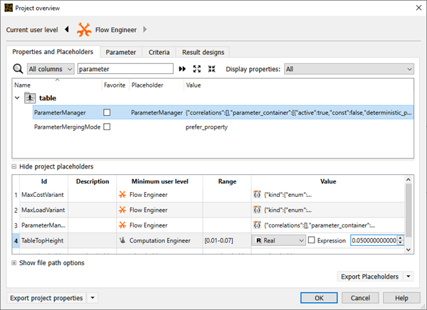
Repeat steps 10-14 to create the following placeholders:
Id Description Minimum user level Range Value TableTopLength Computation Engineer [1-5] Real, 1.8 TableTopWidth Computation Engineer [0.8-1.2] Real, 1.01 TableLegHeight Computation Engineer [0.7-0.9] Real, 0.8 TableLegRadius Computation Engineer [0.01-0.02] Real, 0.015 MaxCosts The maximum accepted costs (Euros) Computation Engineer [0-1000] Real, 300.1 MaxLoad The maximum table load (kg) Computation Engineer [1-500] Real, 50 Double-click the Value cell for row 1 (MaxCostVariant).
Select the Expression check box.
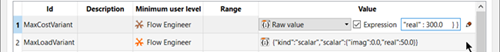
Click
 (Edit
expression).
(Edit
expression).Replace
300with the placeholder value$(MaxCosts).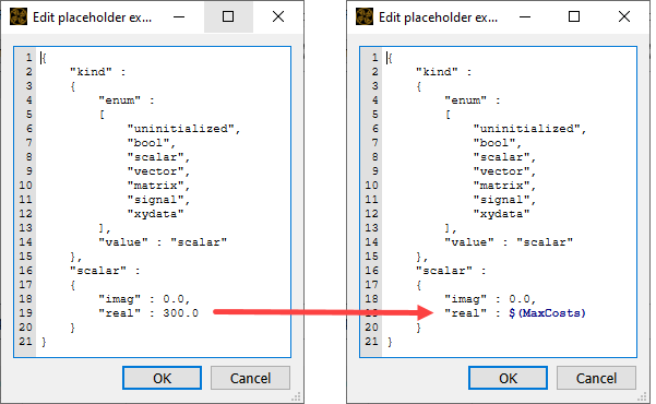
Click .
Repeat steps 16-20 for MaxLoadVariant.
Double-click the Value cell for row 3 (ParameterManager).
Select the Expression check box.
Click
(Edit
expression).Switch to the Text view tab.
Replace table_top_height reference value of
0.05with the placeholder valueTableTopHeight.Replace table_top_length reference value of
1.8with the placeholder valueTableTopLength.Replace table_top_width reference value of
1with the placeholder valueTableTopWidth.Replace table_leg_height reference value of
0.8with the placeholder valueTableLegHeight.Replace table_leg_radius reference value of
0.015with the placeholder valueTableLegRadius.Click .
To save the placeholders, click .
Complete one of the following, depending on which storage location option you selected in the application wizard:
: Add the wizard in optiSLang Web Service
: In the optiSLang Web Service user interface, update the Wizard pane and run the application.