This tutorial allows you to complete signal analysis and signal metamodels with Statistics on Structures.
This tutorial demonstrates how to do the following:
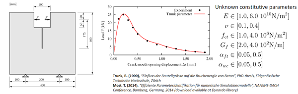
Use the results of a sensitivity analysis of a wedge splitting test with signal-type (xy-data) responses
Create a signal Metamodel of Optimal Prognosis (MOP) node
Perform calibration based on the MOP solver
This tutorial requires optiSLang 3D Post-Processing (oSP3D) version 2021 R1 or later and a valid oSP3D; license.
Before you start the tutorial, download the signal_mop zip file from here , and extract it to your working directory.
To set up and run the tutorial, perform the following steps:
Start optiSLang.
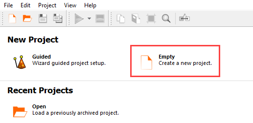
Create a new empty project.
This tutorial provides instructions for manually connecting input and output slots. To display the slots in the node flyouts, from the menu bar select > > .
Under Modules, expand and .
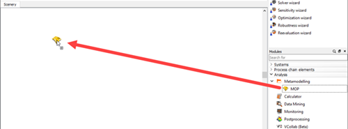
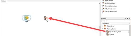
Drag a MOP node onto the Scenery pane and let it drop.
Double-click the MOP node.
To the right of the Absolute path field, click the orange folder.
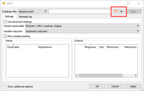
Browse to the signal_mop folder and select Sensitivity.omdb.
Click Open.
Select the Use advanced settings check box.
In the Advanced Settings tab, expand Models and Signal MOP.
Select the True check box.
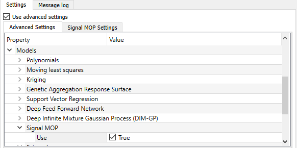
To close the dialog box, click .
To save the project, click
 .
.Browse to the location to save the project and type a project name in the File name field.
Click .
To run the project, click
 .
.
Right-click the MOP node and select from the context menu.
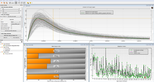
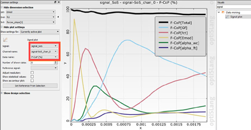
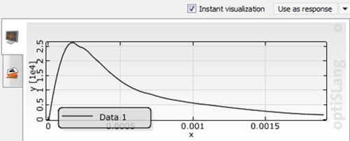
In the Visuals pane, search for and select a signal plot.
From the Signal list, select .
The F-CoP values (in percentages) are displayed.
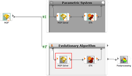
Under Modules, expand and .
Drag a Parametric System node onto the Scenery pane.
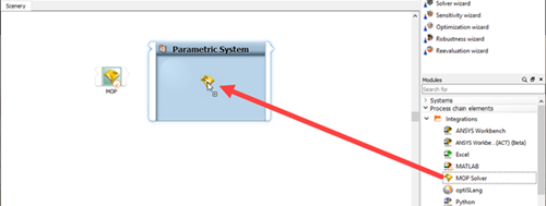
Under Modules, expand and .
Drag a MOP Solver node onto the Parametric System.
Select the Receive design from parent system and Send design back to parent system check boxes.
Click .
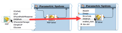
Hover over the right side of the MOP node.
Click OMDBPath and drag it onto IMDBPath on the left side of the MOP Solver node.
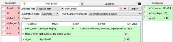
Double-click the MOP Solver node.
Verify that the parameter and response registration is complete as shown in the following image.
Click .
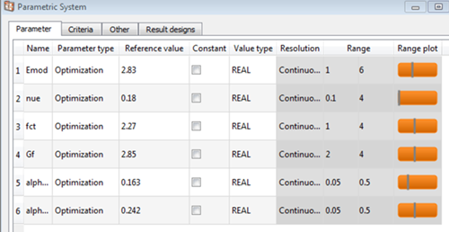
Double-click the Parametric System.
Verify that the parameter properties are set as shown in the following image.
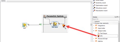
Under Modules, expand and .
Drag a ETK node onto the output connection of the MOP Solver node.
Double-click the ETK node.
Click .
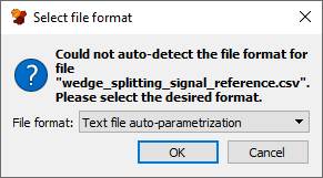
In the Choose a file to open dialog box, browse to the signal_mop folder and select wedge_splitting_signal_reference.csv.
Click .
From the File format list, select and click .
Select as the search mode.
Drag wedge_splitting_signal_reference to the Responses pane to register it as a response.
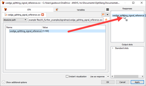
Click .
To save the project, click
.To run the project, click
.
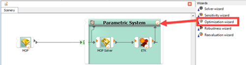
From the Wizards pane, drag the Optimization wizard to the Parametric System and let it drop.
Do not adjust the current parameter properties.
Click .
Click Objective.

In the Criteria pane, double-click the Expression cell and type
euklidnorm(signal - interpolate(wedge_splitting_signal_reference, extract(signal,0))).Click .
Click .
Select Evolutionary Algorithm (EA) as the optimization method.
Click .
Do not adjust the default additional options.
Click .
Click OMDBPath and drag it onto IMDBPath on the left side of the Evolutionary Algorithm MOP Solver node.