This tutorial allows you to perform a sensitivity analysis of the Kursawe functions.
This tutorial demonstrates how to do the following:
Define the Design of Experiment (DOE) scheme
Perform a sensitivity analysis including Metamodel of Optimal Prognosis (MOP)
Extend the data base by the adaptive MOP
Remove outliers and rebuild the MOP
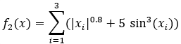
The Kursawe Functions
Objective function one has one dominant global optimum. Objective function two has four local optima.

You must complete the Process Integration of Kursawe Functions tutorial before starting this one.
To set up and run the tutorial, perform the following steps:
Start optiSLang.
From the Start screen, click .
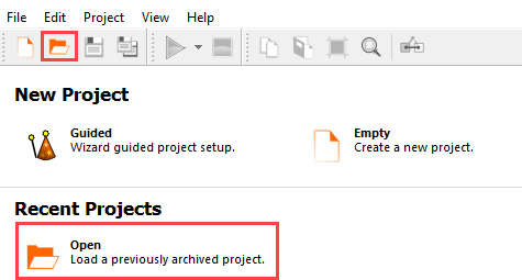
Browse to the location of the Kursawe process integration project you created in the previous tutorial and click .
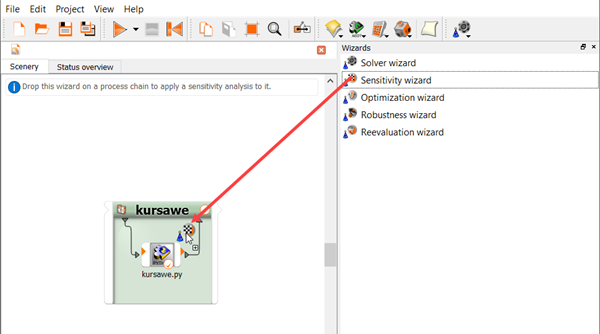
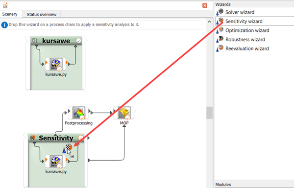
From the Wizards pane, drag the Sensitivity wizard to the kursawe system and let it drop.
Do not adjust the values in the Parametrize Inputs table.
Click .
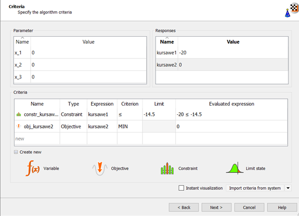
Drag kursawe1 to the Constraint Less icon.
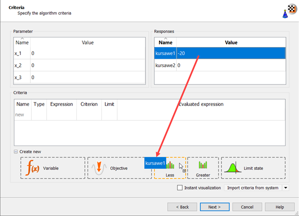
The new criterion appears in the Criteria table.
Change the kursawe1 Limit field to
-14.5.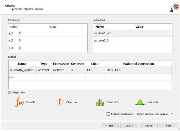
Drag kursawe2 to the Objective Minimize icon.
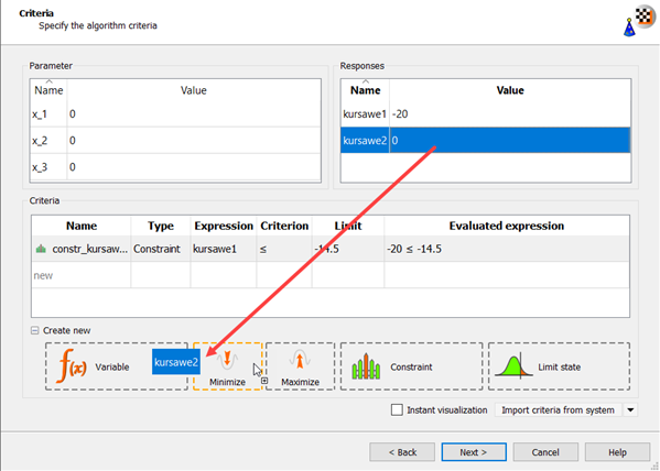
The new criterion appears in the Criteria table.
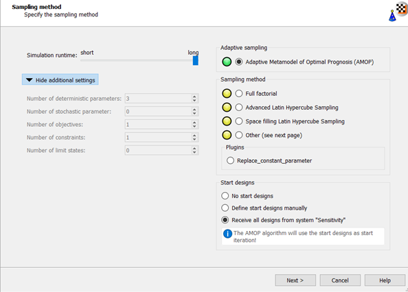
Click .
Select the Space filling Latin Hypercube Sampling method.
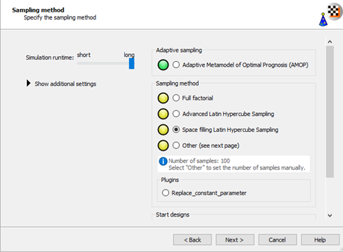
Click .
Do not adjust the current postprocessing settings.
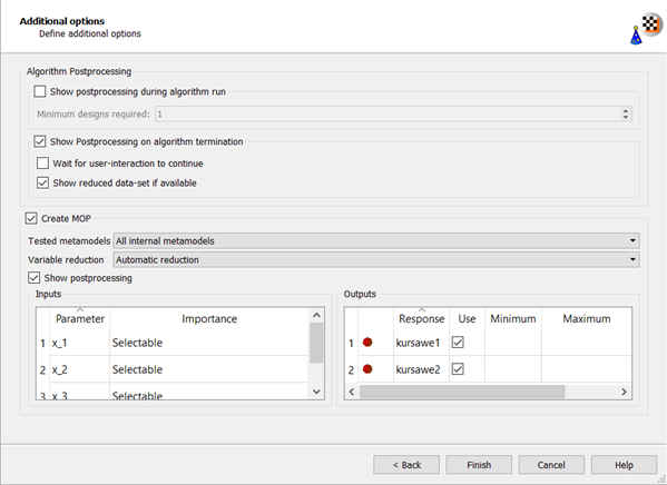
Click .
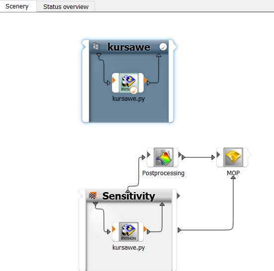
The sensitivity flow is displayed on the Scenery pane.
To save the project, click
 .
.To start the sensitivity analysis, click
 .
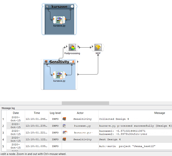
.The bar on top of the sensitivity system displays the progress of the analysis. The message log displays the sequence of events.
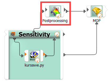
To open the postprocessing results, double-click Postprocessing.
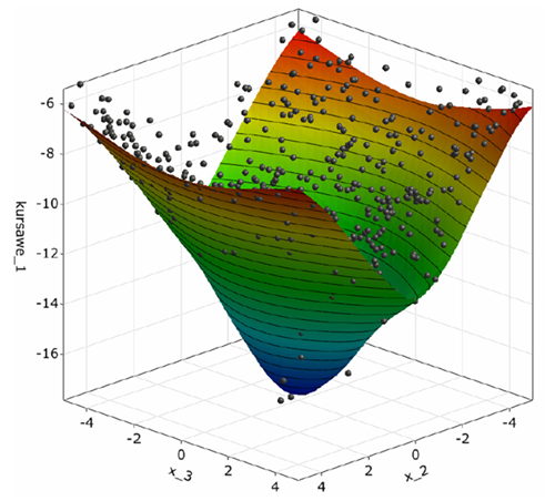
The postprocessing shows a 3D-subspace-plot of the approximation function depending on the two most important parameters.
Function one is approximated very well.
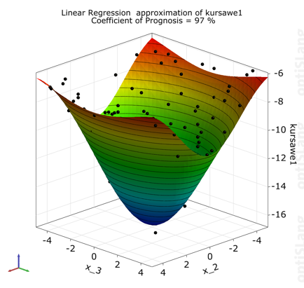
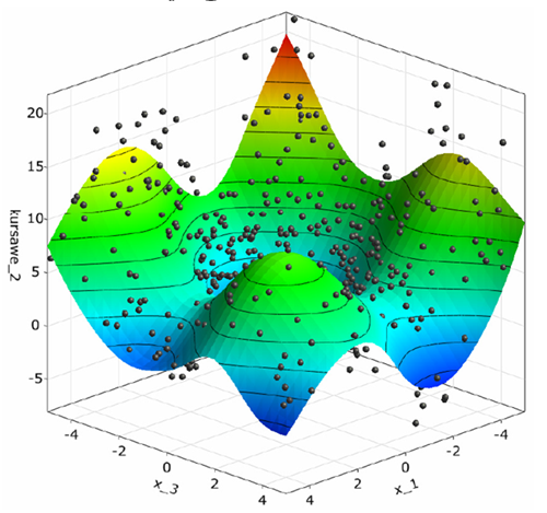
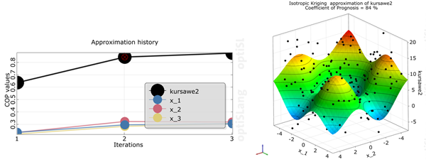
Function two has law prognosis quality due to strong nonlinearities, but general behavior and local optima can be represented sufficiently.
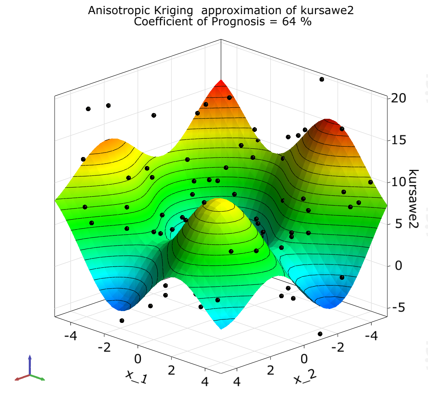
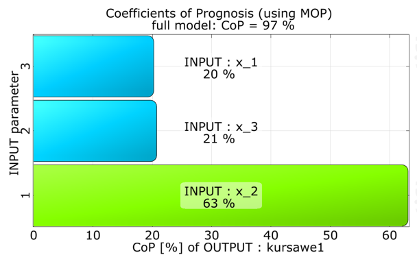
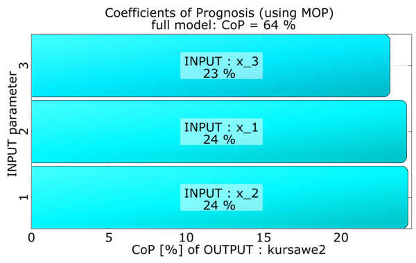
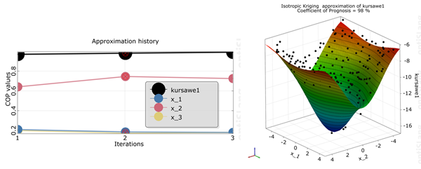
The approximation quality in terms of the Coefficient of Prognosis is shown together with the variance contribution of the single variables.
Function one is mainly influenced by x_2.
Function two is equally influenced by all three variables.
To increase the data set, drag and drop the sensitivity wizard onto the head of the Sensitivity system.
Leave the sampling method settings at the default and click .
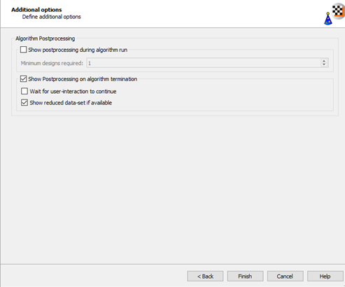
Leave the additional optional settings at the default and click .
An AMOP system is displayed on the Scenery pane.
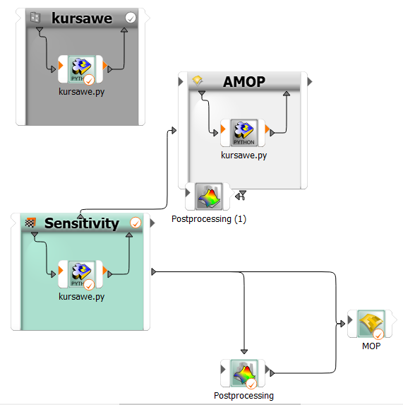
The designs of the first sensitivity system are automatically considered as start designs for the following AMOP using a slot connection.
Double-click the AMOP system to open the settings.
On the Adaption tab, select the check box.
In the Target CoP field, enter
0.99(set target to 99%).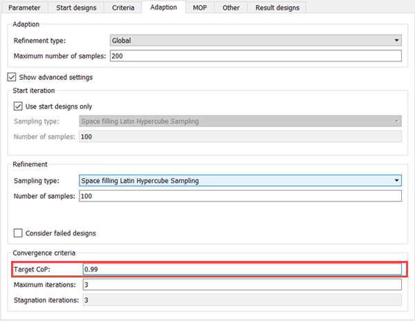
To save and close the settings, click .
To save the project, click
.To run the project, click
.The AMOP postprocessing is displayed. You can observe:
kursawe1
The Coefficient of Prognosis was increased to 98% in 3 iterations
The influence of the individual parameters was changed
The AMOP stopped by reaching the maximum number of iterations
kursawe2
The Coefficient of Prognosis was increased to 84% in 3 iterations
The influence of the individual parameters was changed slightly
The AMOP stopped by reaching the maximum number of iterations
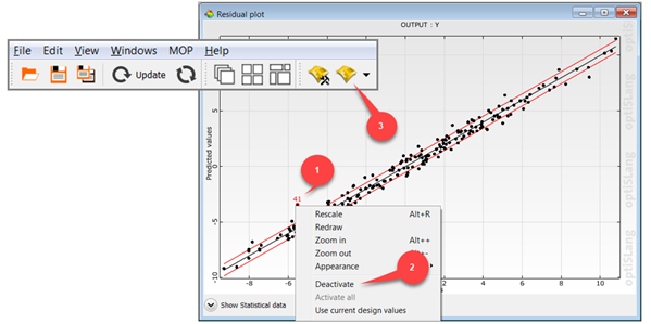
The residual plot shows the predicted values (from cross validation) versus the original data values by indicating lower and upper error bounds. Error bounds are obtained from the standard deviation of the error values multiplied with the user defined sigma level. Samples outside the error bounds may be possible outliers.
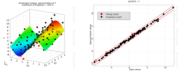
To deactivate outliers:
Select outliers in the residual plot.
Right-click and select from the context menu.
To update the MOP directly in the postprocessing, click
 .
.