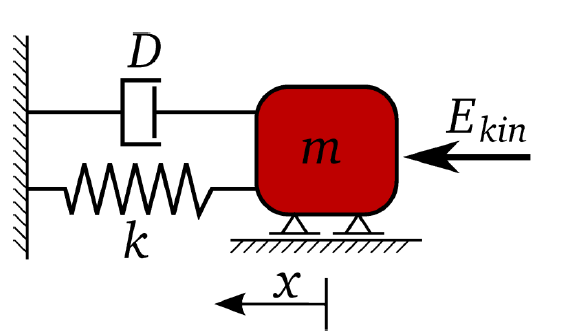
This tutorial allows you to complete a calibration of a single degree-of-freedom system excited with initial kinetic energy.

The equation of motion of free vibration is:

The un-damped and damped eigen-frequency is

The time-dependent displacement function is:

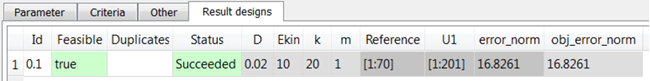
The goal is the identification of the input parameters m, k, D, and Ekin to optimally fit a reference displacement function.

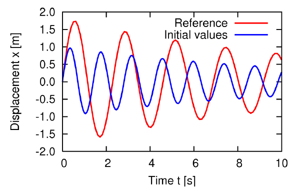
The objective function is the sum of squared errors between the reference and the calculated displacement function values

This tutorial demonstrates how to do the following:
Generate a solver chain using ABAQUS
Define the input parameters
Define the output and reference signals
Before you start the tutorial, download the oscillator_signals_abaqus zip file from here , and extract it to your working directory.
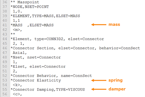
The spring mass system is coded in the supplied input script for ABAQUS named oscillator.inp.
To set up and run the tutorial, perform the following steps:
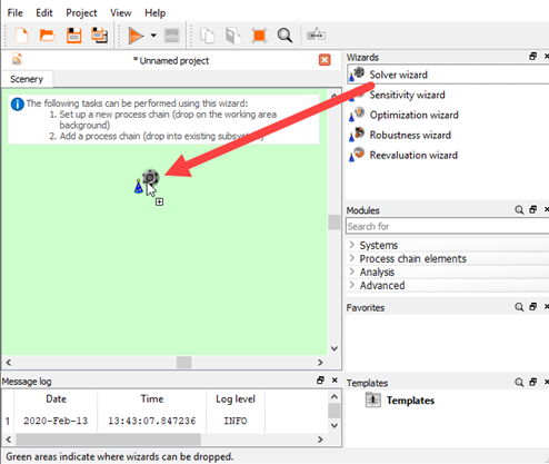
- Creating a New Project
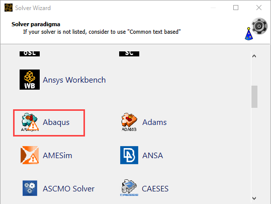
- Starting the Solver Wizard
- Selecting the Input File
- Defining the Input Parameters
- Editing the Parameter Properties
- Selecting the Output Data File
- Defining the Output Data
- Selecting the Reference Data File
- Defining the Reference Signal
- Defining the Signal Functions
- Defining the Optimization Criteria
- Defining the Solver Process
- Creating the Solver Chain Template
- Saving and Running the Project
From the Wizards pane, drag the Solver wizard to the Scenery pane and let it drop.
From the solver list, click .
In the Select input file dialog box, browse to the oscillator_signals_abaqus folder and select oscillator.inp.
Click .
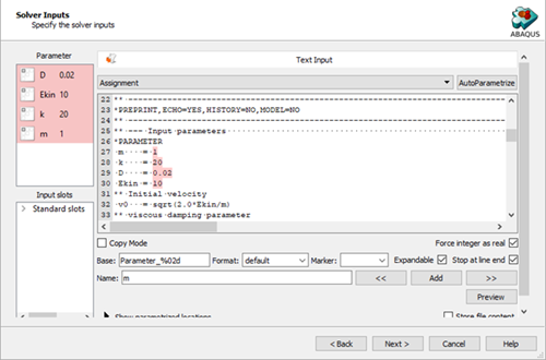
In the text editor, highlight lines 27-30
Select the AutoParametrize mode.
Click .
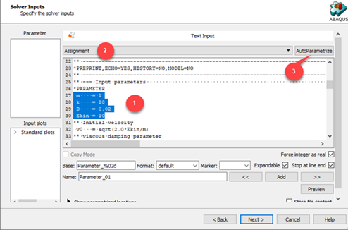
All possible values are marked.
Change the parameter name to
m.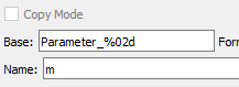
To register the parameter, click Add.
Repeat this procedure for parameters k, D, and Ekin.
Click .
Double-click the range numbers for row 1 (m).
Change the lower bound to
0.1and the upper bound to5.Double-click the range numbers for row 2 (k).
Change the lower bound to
10and the upper bound to50.Double-click the range numbers for row 3 (D).
Change the lower bound to
0.01and the upper bound to0.05.Double-click the range numbers for row 4 (Ekin).
Change the lower bound to
10and the upper bound to100.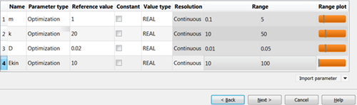
Click .
In the Choose a file to open dialog box, browse to the oscillator_signals_abaqus folder and select oscillator.odb.
Click .
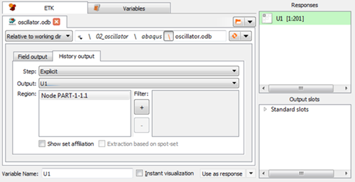
Switch to the History output tab.
From the Output list, select .
In the Variable Name field, type
U1.Click .
The output is added to the Responses pane.
To open the reference data file, click the orange folder.
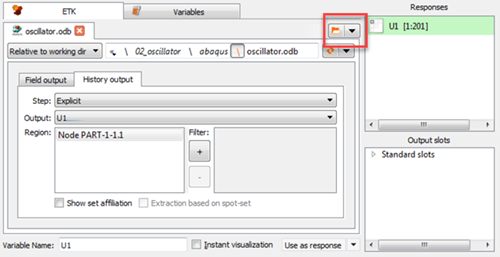
In the Choose a file to open dialog box, browse to the oscillator_signals_abaqus folder and select oscillator_reference.txt.
Click .
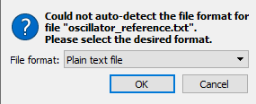
From the File format list, ensure is selected and click .
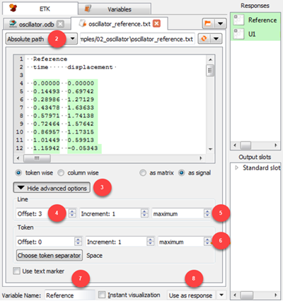
Select as the search mode.
Expand Show advanced options.
Under Line, set
Offset: 3.Set the number of lines to
maximum.Set the number of tokens to
maximum.In the Variable Name field, type
Reference.Click .
The signal is displayed in the Responses pane.
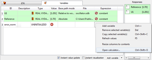
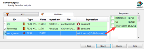
Switch to the Variables tab
In row 2 (Reference), double-click the Base path mode cell and select from the drop-down list.
Click .
Double-click the ID cell for the new variable, type
error_norm, and press Enter.Right-click the Expression cell of row 3 (error_norm) and select from the context menu.
In the calculator, switch to the Linear Algebra tab.
Click .
In the brackets, type
U1-Reference.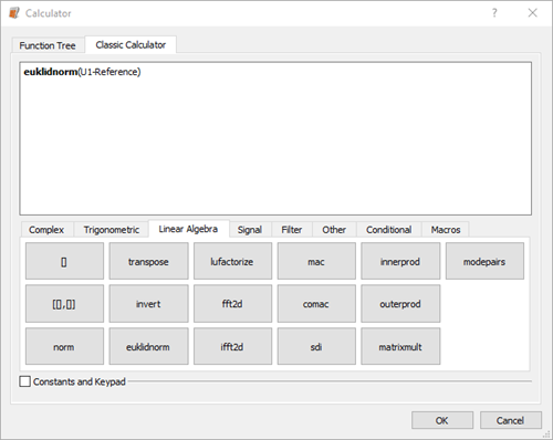
Click .
Drag the error_norm row into the Responses pane to register it as a response.
Select the Instant visualization check box and compare the two signals in the diagram to make sure that there is not a time unit or scaling error.
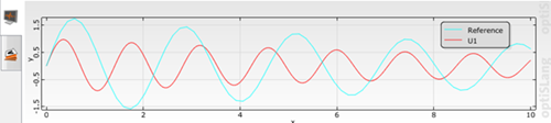
Click .
To define error_norm as a minimization objective, drag the row from the Responses table to the Objective Minimize icon and let it drop.
The new criterion is displayed in the Criteria table.
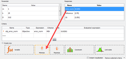
Click .
Select the Create a template from solver chain check box.
In the Template name field, enter
oscillator_calib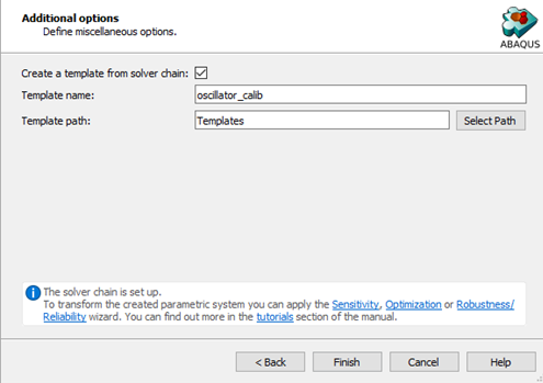
Click .
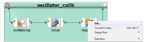
The template is displayed in the Scenery pane.


Note: This is an optional procedure.
Right-click the Output files node and select from the context menu.
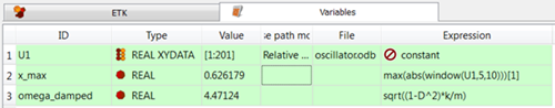
Define the x_max variable, using the window function.
Define the omega_damped variable, which is not readily present in the ABAQUS results file.
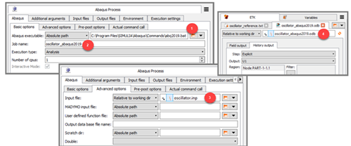
Note: This is an optional procedure.
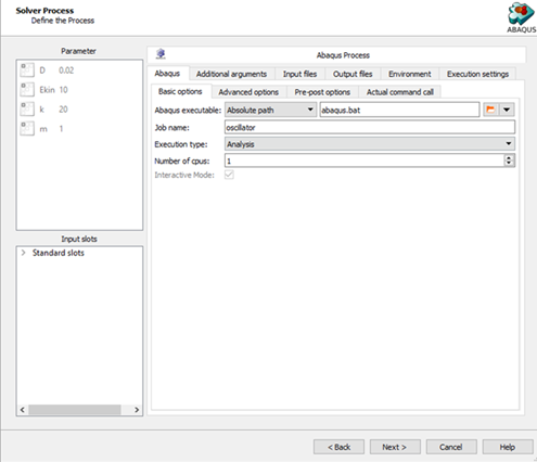
Select the ABAQUS executable.
Create a job name which differs from the input file name.
Specify the input file name.
Set the output file (jobname.odb) as the result for data extraction.
Note: You many need to modify the output files as well if changes apply to a wizard generated node.