Calibration of a Damped Oscillator in Ansys Workbench

This tutorial allows you to complete a calibration of a single degree-of-freedom system excited with initial kinetic energy.

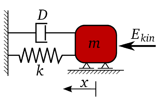
The equation of motion of free vibration is:

The un-damped and damped eigen-frequency is

The time-dependent displacement function is:

In this tutorial, you complete the calibration using the optiSLang extension in Workbench.

Problem Definition

The goal is the identification of the input parameters m, k, D, and E_kin to optimally fit a reference displacement function.

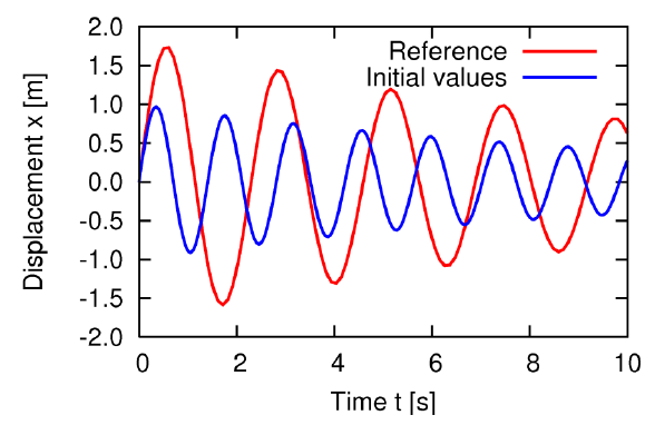
The objective function is the sum of squared errors between the reference and the calculated displacement function values

Task Description

This tutorial demonstrates how to do the following:

Generate a solver chain using Ansys Workbench and optiSLang signal processing
Define the input parameters
Define the output and reference signals
Perform a sensitivity analysis of signal extraction terms using the given parameter bounds
Complete a single, objective, unconstrained optimization by minimizing the sum of squared errors over all time steps

Preparation

Before you start the tutorial, download the oscillator_optimization_calibration_workbench zip file from here , and extract it to your working directory.

If you do not see an optiSLang section in the Workbench Toolbox, ensure that the Ansys Workbench optiSLang Extension is installed and activated.

Tutorial Steps

To set up and run the tutorial, perform the following steps:

Opening the Workbench Project

Start Workbench.
From the menu bar, select File > Open.
Browse to the oscillator_optimization_calibration_workbench folder and select oscillator_apdl.wbpz.
Click Open.
To save the archive file as a Workbench project file, click Save.
To update the project, click .

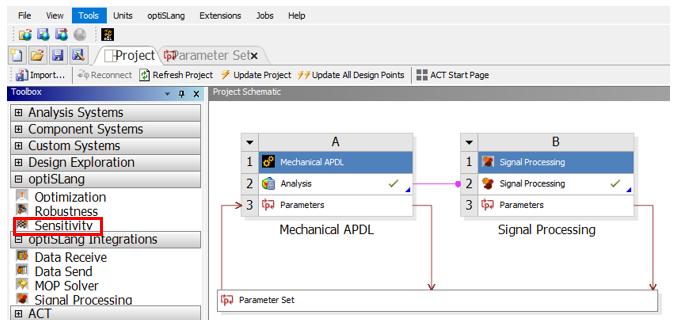
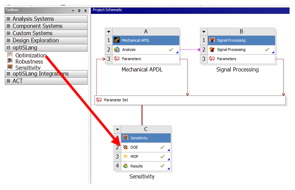
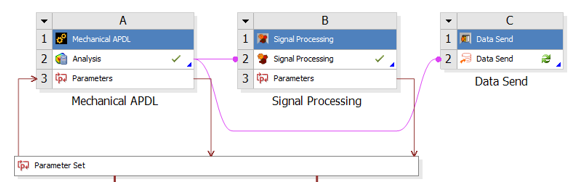
Connecting a Signal Processing System

Drag the Signal Processing system from the Toolbar and drop it onto the Analysis cell of the Mechanical APDL system.
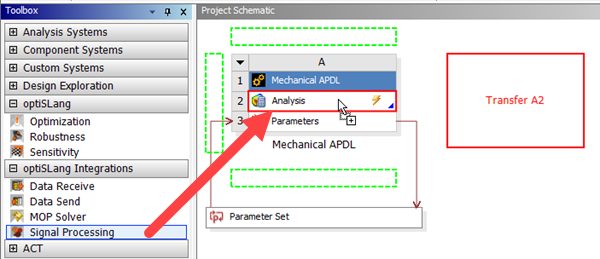
The Signal Processing system is added to the Project Schematic.

Selecting the Solver Signal File

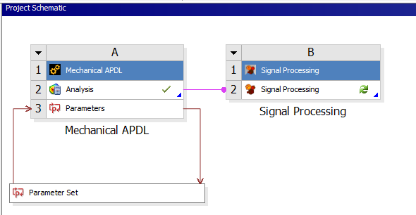
Double-click the Signal Processing cell of the Signal Processing system.
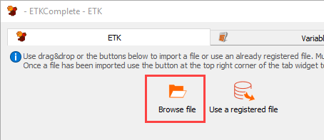
On the ETK tab, click Browse file.
In the Choose a file to open dialog box, browse to the oscillator_optimization_calibration_workbench\oscillator_apdl_files\dp0\APDL\ANSYS folder and select oscillator_signal.txt.
Click Open.

Defining the Solver Signal

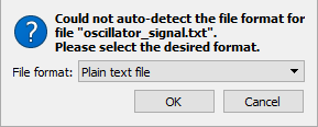
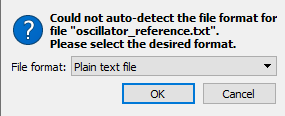
From the File format list, ensure Plain text file is selected and click OK.
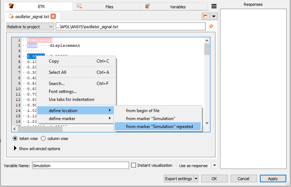
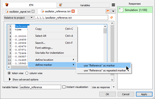
Highlight the text in line 1 (Simulation).
Right-click the selection and select define marker > use "Simulation" as marker from the context menu.
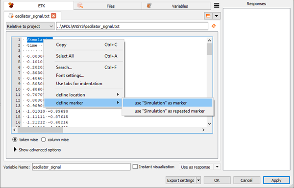
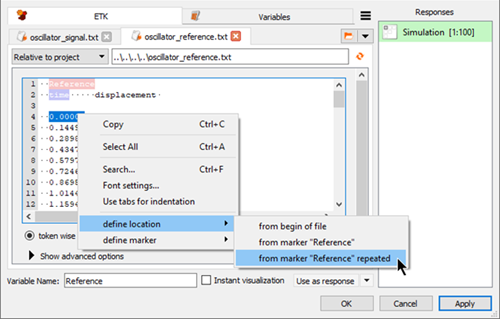
Highlight the first number in line 4 (0.00000)
Right-click the selection and select define location > from marker "Simulation" repeated from the context menu.
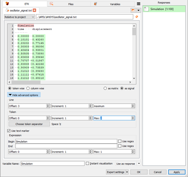
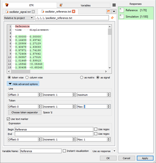
Expand Show advanced options.
Under Token, set Max: 2.
Click Use as response.
The signal is displayed in the Responses pane.
You can select the Instant visualization check box to see if the response is extracted correctly.

Selecting the Reference Signal File

To open the reference signal file, click the orange folder.
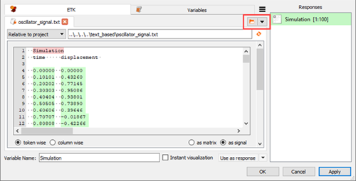
In the Choose a file to open dialog box, browse to the oscillator_optimization_calibration_workbench folder and select oscillator_reference.txt.
Click Open.

Defining the Reference Signal

From the File format list, ensure Plain text file is selected and click OK.
Highlight the text in line 1 (Reference).
Right-click the selection and select define marker > use "Reference" as marker from the context menu.
Highlight the first number in line 4 (0.00000).
Right-click the selection and select define location > from marker "Reference" repeated from the context menu.
Expand Show advanced options.
Under Token, set Max: 2.
Click Use as response.
The signal is displayed in the Responses pane.

Defining the Signal Functions

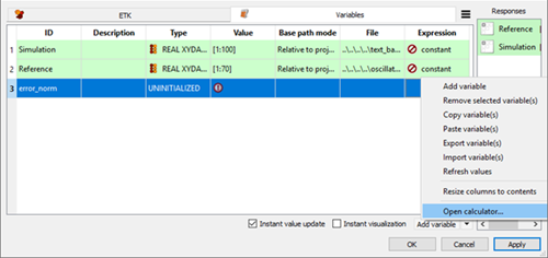
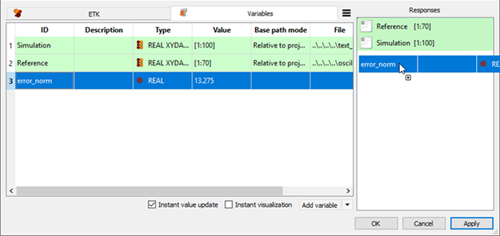
Switch to the Variables tab
Click Add variable.
Double-click the ID cell for the new variable, type error_norm, and press Enter.
Right-click the Expression cell of row 3 (error_norm) and select Open Calculator from the context menu.
In the calculator, switch to the Linear Algebra tab.
Click euklidnorm.
In the brackets, type Simulation-Reference.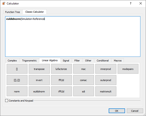
Click OK.
Drag the error_norm row into the Responses pane to register it as a response.
Click OK.
To save the current project, from the menu bar, select File > Save or from the main toolbar, click .
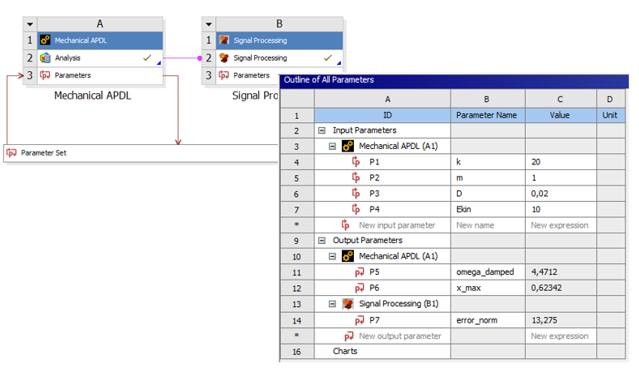
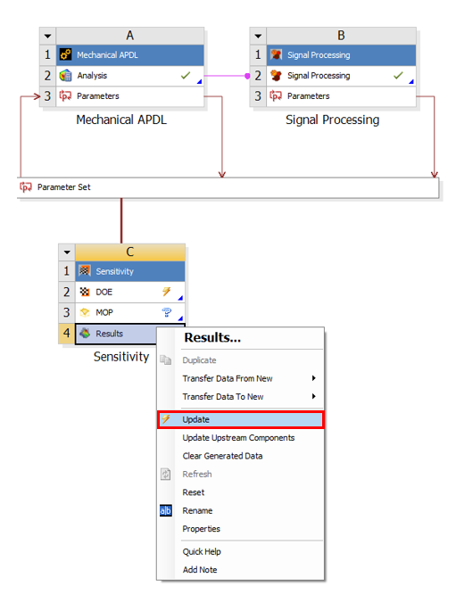
Right-click the Signal Processing cell of the Signal Processing system and select Update from the context menu.
After updating the project, the additional scalar response is displayed in the parameter set.

Completing the Sensitivity Wizard

To start a new sensitivity analysis, in the Workbench Toolbox, double-click the Sensitivity system.
Double-click the range numbers and set the following:
Row Lower Bound Upper Bound
k 10 50
m 0.1 5
D 0.01 0.05
Ekin 10 100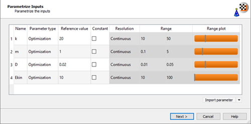
Click Next.
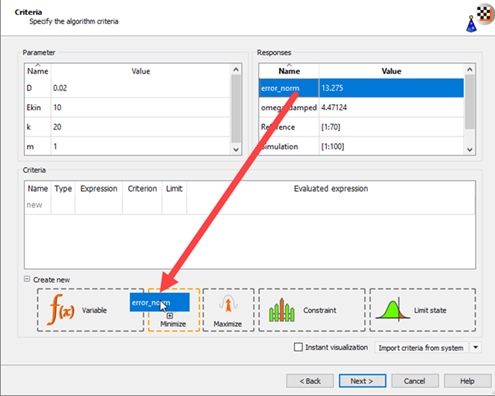
To define error_norm as a minimization objective, drag the row from the Responses table to the Objective Minimize icon and let it drop.
The new criterion is displayed in the Criteria table.
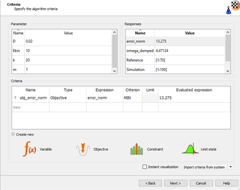
Click Next.
Change Simulation runtime to short.
Select the Space filling Latin Hypercube Sampling sampling method and leave the number of samples at 100.
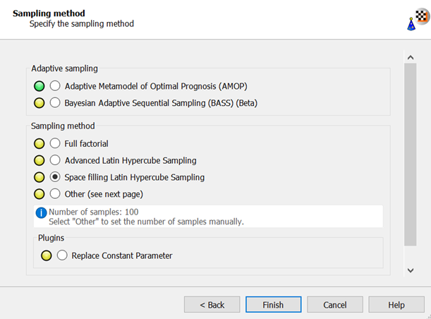
Click Finish.

Row	Lower Bound	Upper Bound
k	10	50
m	0.1	5
D	0.01	0.05
Ekin	10	100

Running the Sensitivity Analysis

To save the current project, from the menu bar, select File > Save or from the main toolbar, click .
Right-click the Results cell of the Sensitivity system and select Update from the context menu.
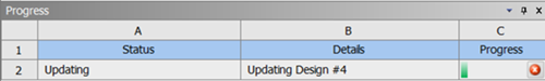
The DOE is created in the background and all designs are calculated.
The Progress pane displays the status of the update and a progress bar.
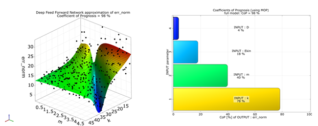
Finally, the MOP is generated and the signal data is displayed.
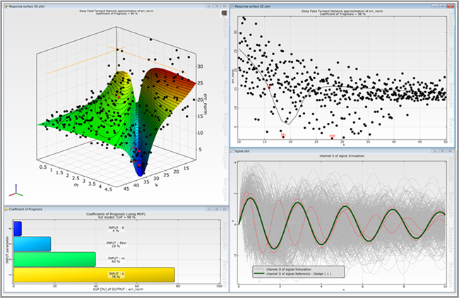
You can observe that there is a highly non-linear relationship between input parameters and the error norm and significant influence of mass (m) and spring constant (k).

Completing the Optimization Wizard

Drag the Optimization wizard from the Toolbar and drop it onto the DOE cell of the Sensitivity system.
Do not adjust the values in the Parametrize Inputs table.
Click Next.
Do not adjust or add to the currently displayed values for parameters, responses, and criteria.
Click Next.
Click Manual optimizer selection.
Select the Downhill Simplex Method optimization method.
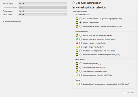
From the Analysis status list, select Preoptimized.
Click Finish.
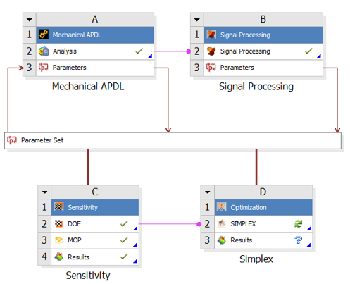
The Optimization system is added to the Project Schematic.

Running the Simplex Optimization

To save the current project, from the menu bar, select File > Save or from the main toolbar, click .
Right-click the Results cell of the Optimization system and select Update from the context menu.
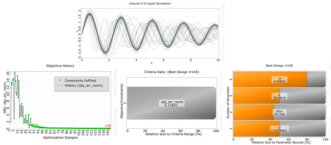
The Simplex converges well to a small signal difference.

Viewing Images in the Post Processor

Note: This is an optional procedure.

Drag the Data Send module from the Toolbar and drop it onto the Analysis cell of the Mechanical APDL system.
The Data Send system is added to the Project Schematic.
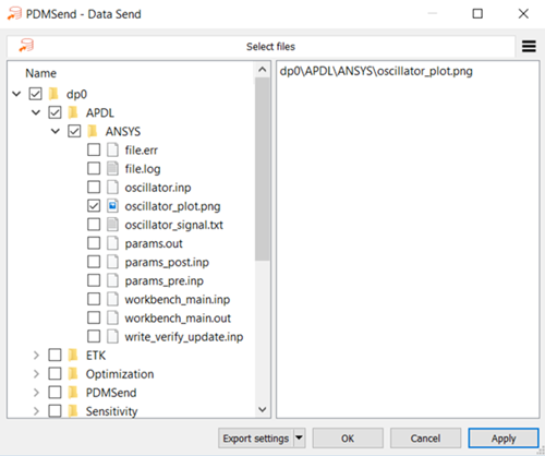
Double-click the Data Send system Setup cell.
In the left pane, select the solver images to copy to the design directory.
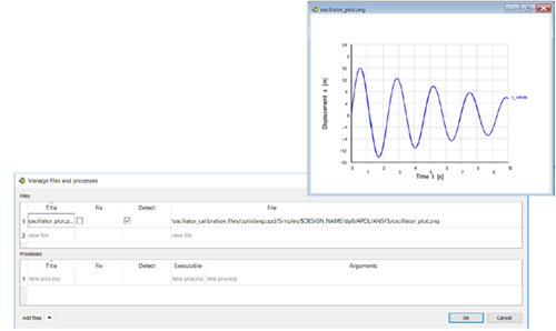
Double click the Results cell of the Sensitivity or Optimization systems to view the postprocessing.
In the optiSLang postprocessing Monitoring pane, select Edit > External files and processes.
Select the image from an arbitrary design directory.
The image of the currently selected design is displayed.