This multi-part tutorial, which assumes that you are familiar with Mechanical, shows how to create geometric imperfections on parts of a model's surface in Ansys Mechanical using the oSP3D extension. The tutorial uses a synthetic random field to introduce geometry displacements on a named selection of surfaces. The variation of the field of geometric imperfections is controlled with a number of scalar parameters, which are added to the parameter list of the Mechanical model.
This example simulates the stress field in a simple steel cube. The cube is assumed to be permanently attached to a solid horizontal surface. A constant uniform force acts perpendicular to one side. The cube's bottom face forms a fixed support. The flat geometry of the surface on which the constant uniform force acts is modified by the synthetic random field.
This tutorial consists of:
To create a synthetic random field:
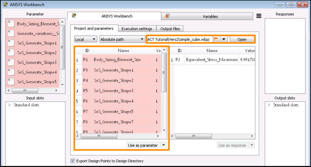
In Ansys Workbench, open the archive file simple_cube.wbpz in
oSP3D_examples\ansys\simple_cube.Rename the project file as simple_cube_tutorial2 and save it in the same folder.
If you see a message indicating that the oSP3D extension will be upgraded permanently when you save the project, click .
This project contains a Static Structural system that calculates stress and deformation.
Set up and solve the Mechanical model.
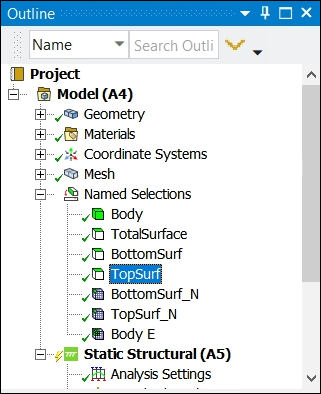
This model contains named selections.
In the Mechanical ribbon, select >
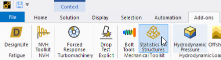
From the oSP3D tab, select > .
A Synthetic random field (SoS) node is added to the system.
You can now configure this node.
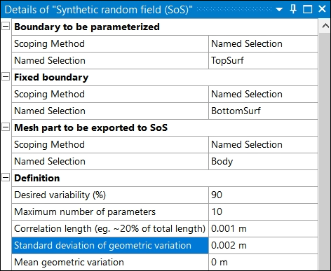
In the details for the Synthetic random field (oSP3D) node:
Set Boundary to be parametrized to the named selection TopSurf.
Geometric imperfections are created on this surface.
Set Fixed boundary to the named selection BottomSurf.
A fixed boundary must be defined as oSP3D performs mesh or grid morphing in reference to this fixed part of the mesh or grid.
Note: Best practice is to ensure that there are free nodes between the fixed and parametrized boundary. This helps with a smooth transition from the fixed parts to the morphed parts of the geometry.
Set Mesh part to be exported to oSP3D to the named selection Body.
Geometric imperfections are created on this surface.
Tip: To save computation time in oSP3D, export a substructure.
Set Correlation length to 0.001 m.
Set Standard deviation of geometric variation to 0.002 m.
You can now generate and visualize the synthetic random field.
To generate and visualize the synthetic random field:
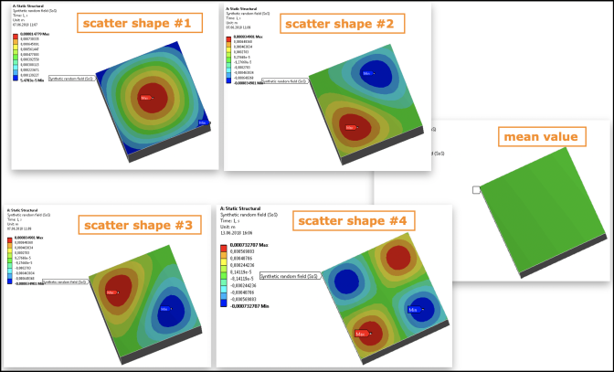
Right-click the Synthetic random field (SoS) node and select .
In the details for the Synthetic random field (oSP3D) node, under Visualization, set Visible variation shape index (0=mean) to a scatter shape of your choice.
This image shows the first four and mean scatter shapes of the synthetic random field.
You can now set some advanced options.
In the details for the Synthetic random field (SoS) node, set these advanced options:
- Use mesh stabilization
Setting this option to True makes the mesh morphing more robust, allowing you to create larger deformations. The mesh is stabilized iteratively to avoid element distortions that are too large. Computation time may increase substantially.
- Test on mesh distortion
Setting this option to True has oSP3D perform a strict test for excessive mesh distortion before calling the Mechanical solver. Using this option avoids starting unnecessary long-running simulations.
Note: This test is stricter than Mechanical's test.
- Move nodes along
Setting this option to Boundary normal applies mesh morphing perpendicular to the boundary.
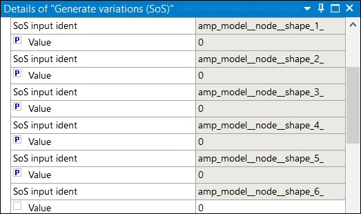
You can now configure the Generate variations (SoS) node.
In the details for the Generate variations (SoS) node:
Under Input parameters, select the amplitude values of your choice.
The synthetic random field of imperfections calculated are visualized after solving the project.
Caution: Large amplitude magnitudes (greater than 1) may lead to failed mesh morphing.
Set the check boxes for the first five shape amplitude parameters.
This registers them in the Workbench Parameter Set, making them available for parametrization in optiSLang.
Note: Selecting more amplitude parameters leads to a more detailed variation of geometric imperfections.
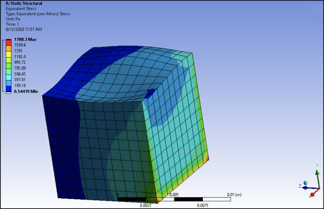
Solve the model.
This image shows a mesh morphed according to the generated synthetic random field of distortions.
Save and close your Workbench project.
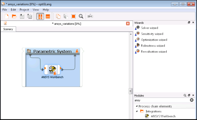
You can now perform a robustness analysis in optiSLang.