


In variance-based robustness analysis the variations of the critical model responses are investigated. In optiSLang random sampling methods are used to generate discrete samples of the joined probability density function of the given random variables. Based on these samples, which are evaluated by the solver similarly as in the sensitivity analysis, the statistical properties of the model responses as mean value, standard deviation, quantiles and higher order stochastic moments are estimated. In order to obtain a sufficient quality of these estimates, it is required, that the sampling scheme represents the marginal distributions of the single random variables as well as the defined correlations between each other with high accuracy. Some very basic stochastic methods to generate sample sets are variants of the Monte-Carlo method. The simplest version is the so-called plain Monte-Carlo method (PMC). With this methods the natural scatter can be modeled quite well, but the statistical uncertainty is fairly large if the sample size is small. Therefore optiSLang provides Latin Hypercube Sampling (LHS) with minimized correlation errors (Hungtington and Lyrintzis 1998), where the marginal distributions and the predefined input correlations are represented with a small number of samples.
Based on the estimates of the mean value and the standard deviation the safety margin can be estimated by using Equation 4–1 for the responses where a performance limit is given. However, by using variance-based robustness analysis only safety margins up to two sigma can be proven with a small number of samples. For larger safety margins (e.g. six sigma) the true failure rate may be heavily vary for different distribution types of the output. Since the distribution of the output is not exactly known, an estimate of low failure probabilities by variance-based measures may be very inaccurate. Therefore, safety margins larger than three sigma should be proven by reliability analysis.
Additional to the variation of the response, the mean value could be an indicator regarding the robustness of a design. If the mean value estimated by the samples strongly differs from the deterministic reference value, the influence of the input uncertainties and potentially of solver inaccuracies is significant.
|
|
|
Representation of a noisy model output by a smoothing approximation (left) and convergence behavior of the explained variation in the case of a robust and non-robust model (right). |
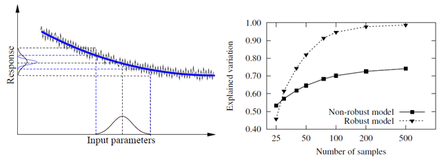
In order to quantify the sources of the response variation, in optiSLang variance-based sensitivity measures are estimated within the robustness analysis. For this purpose the Meta-model of Optimal Prognosis presented in Metamodel of Optimal Prognosis is applied. If the solver output contains unexplainable effects due to numerical accuracy problems, the MOP approximation will smooth these noise effects as shown in Figure 4.5: Noisy Model Outpot and Convergence Behavior. If this is the case, the CoP value of the MOP can be used to estimate the noise variation as the shortcoming of the CoP to 100% explainability. However, the unexplained variation may not be caused by solver noise only, but also by a poor approximation quality. This problem should be analyzed by increasing the number of samples in the case of low explainability. If the CoP does not increase, then this is an indicator for unexplainable solver behavior.
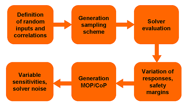
In Figure 4.6: Flowchart of Variance-Based Robustness Analysis Available in optiSLang, the overall flow of the variance-based robustness analysis provided by optiSLang is illustrated. Based on the initial definition of random variables, optimized samples are generated and evaluated by the solver. The solver results are used to estimate the statistical properties and to perform a sensitivity analysis with help of the MOP approach. If the design does not fulfill the robustness requirements, the sensitivity indices help to identify these input variables, where a reduction of the uncertainty is most effective with respect to the variation of the model responses.
Exemplary, the variance-based robustness evaluation is performed at the deterministic optimum of the damped oscillator introduced in Single-Objective Optimization. The mass m, the spring stiffness k, the damping ratio D and the initial kinetic energy Ekin are considered as independent random variables. Their mean values and coefficients of variation (CV) are taken as follows
 | (4–10) |
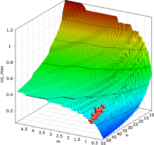
100 Latin Hypercube samples, which are shown in Figure 4.7: Variance-Based Robustness Analysis of the Damped Oscillator, are evaluated. As robustness requirement the safety margin of the mean eigen-frequency to a given limit ωlimit = 8.5 1/s shall be larger or equal 4.5 sigma, which is equivalent to a failure probability of 3.4 · 10−6 for a normal distribution. Furthermore, the mean values and the relative variation of the model responses as well as their explained variations are statistically evaluated.
In Figure 4.8: Statistical Properties of the Oscillator Responses and Input Sensitivities
Obtained with Variance-Based Robustness Analysis the statistical properties of the
maximum amplitude and the damped eigen-frequency are visualized. The figure indicates,
that the coefficient of variation of the maximum amplitude is larger (11%) as the
largest CV of the input variables. Furthermore, the mean value is almost one sigma
larger as the deterministic value ( = 0.25 m). Both facts could be interpreted as indicators for a
non-robust design in terms of the objective.
= 0.25 m). Both facts could be interpreted as indicators for a
non-robust design in terms of the objective.
|
|
|
100 Latin Hypercube samples used for the variance-based robustness analysis of the damped oscillator. |
As result of the MOP-based sensitivity analysis the damping ratio has the largest contribution to the variation of the maximum amplitude. The Coefficient of Prognosis indicates an explained variation of 92% which is smaller as the CoP obtained with the optimization variables, which was 99%. Since the robustness analysis considers in this example a much smaller variation in the random inputs as the sensitivity analysis in the optimization variables, the nonlinearity in the model response should be reduced in the smaller space. The decrease of the CoP in that case indicates an increasing importance of solver noise which is caused by the coarse time discretization of the oscillator response. The statistical evaluation of the damped-eigen-frequency results in a CV of 2.7% which is in the range of the input variation. Furthermore, the CoP indicates an excellent explainability of 100% for this model response. Nevertheless, the require safety margin of 4.5 sigma is not reached. The mean value and the standard deviation given in Figure 4.8: Statistical Properties of the Oscillator Responses and Input Sensitivities Obtained with Variance-Based Robustness Analysis can be used to estimate this safety margin, which is only 2.3 sigma. From the viewpoint of the safety requirements, the design found by the deterministic optimization procedures does not fulfill the robustness criteria. In that case, that the input uncertainties could not be reduced, the optimum should be moved back into the safe region until the safety requirements are fulfilled. This strategy is realized in the Robust Design Optimization presented in the next section.