It is typical for industrial applications to investigate the influence of a large number of random input variables. Modelling these input variables as independent is a simplification, but often the consideration of dependencies between inputs has a significant influence on the results obtained. For example, material properties like the Young’s modulus and yield stress may not vary independently. In optiSLang dependent random variables are modeled with help of the coefficient of correlation

(4–7)

In the following, the random input variables of an investigated model are col- lected in a random vector X. The joint probability density function is used to quantify the probability of a specific combination of values of inputs. In the case that all random variables X_i are independent from each other, then the joint probability density is the product of the single (marginal) density functions.

(4–8)

Note that independent variables are always uncorrelated, while the contrary is not always true. For normally distributed input variables X _g the joint density function reads

(4–9)

where is the vector of mean values, is the covariance matrix and n is the number of random variables. The combination of arbitrary distribution types is not possible in closed form. In optiSLang, the combination of correlated variables with arbitrary distribution types is realized by using the Nataf model (Nataf 1962).

First, the single original random variables are transformed to Gaussian ones. For the assumed joint normal probability density, the coefficients of correlation differ from the original values, they have to be found by iteration. It may happen in special cases that the iteration yields a not positive definite, hence invalid matrix of correlation coefficients. In (Bucher 2009), further details about this procedure can be found.

Figure 4.4: Random Samples of a Two-Dimensional Random Vector

Samples of a log-normal – normal distributed random vector obtained by the Nataf model: in the original space (left) and in the normal space (right).

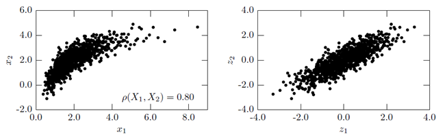
In Figure 4.4: Random Samples of a Two-Dimensional Random Vector, random samples of a two-dimensional random vector with a normal and a log-normal distribution type are shown. The transformed samples in the normal space can be compared to the identical samples in the original space. This indicates, that although linear dependencies are assumed in the normal space, non- linear dependencies can be represented in the original space.