


In single-objective optimization problems the optimization task can be formulated by a single scalar-valued objective function
 | (3–1) |
which is often an implicit function of the design variables. The design variables can
be defined as continuous variables with a lower and upper bound or as discrete variables
which assume several discrete values. In unconstrained optimization prob- lems only the
bounds or values of the design variables limit the optimization space. The optimizer
searches between these limits for the minimum value of the objective function
 . For maximization problems the sign of the user defined objective
function is inverted in optiSLang to get a minimization task.
. For maximization problems the sign of the user defined objective
function is inverted in optiSLang to get a minimization task.
In engineering problems often additional restrictions have to be fulfilled by the optimal design. With help of equality and inequality constraints
 | (3–2) |
such restrictions can be formulated. The constraint functions can represent limitations depending only on the input variables but also depending on all available model responses and any mathematical combination of both.
Equality constraints are very difficult to treat in industrial applications. Therefore, it is not allowed to define equality constraints in optiSLang. However, equality constraints fulfilled with a given tolerance can be formulated easily as inequality constraints and in that way they can be handled by all optimization methods available in optiSLang. In order to get an optimal convergence of the optimizer and sufficiently accurate fulfillment of the constraint conditions, it is very useful to scale the objective and the constraint functions to be in a similar range. This can be realized e.g. by using the results of the design exploration.
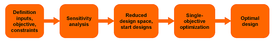
In Figure 3.1: Recommended Flowchart for Single-Objective Optimization, the recommended flow of single-objective optimization procedure is shown: after the definition of the design variables and objective and constraint functions the design space is explored by sensitivity analysis. The obtained variable sensitivities may help to reduce the number of design variables. The best designs found in the sensitivity analysis could be used as start designs for the following optimization procedure which finally will determine an optimal design.
Accompanying Example: Optimization of a Damped Oscillator
The principles of the optimization methods described in the following sections are demonstrated by a simple accompanying example. For this purpose the maximum amplitude of a single degree-of-freedom damped oscillator shown in Figure 3.2: Damped Oscillator: System Properties and Oscillation Behavior shall be minimized.
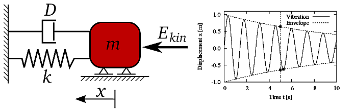
The equation of motion can be formulated depending on the mass m, the spring stiffness k and damping ratio D as follows
 | (3–3) |
where  is the undamped eigen-frequency. Assuming an initial kinetic energy
 and an initial position
  , the time-dependent displacement function can be derived as
follows
, the time-dependent displacement function can be derived as
follows
 | (3–4) |
where  is the damped eigen-frequency. The optimization goal is to minimize
the maximum amplitude after 5 seconds by assuming m and
k as design parameters and D and
as constants
is the damped eigen-frequency. The optimization goal is to minimize
the maximum amplitude after 5 seconds by assuming m and
k as design parameters and D and
as constants
 | (3–5) |
As optimization constraint, the damped eigen-frequency shall be limited: w ≤ 8 1/s.
If the maximum amplitude after 5 seconds is estimated from the envelope curve shown in Figure 3.2: Damped Oscillator: System Properties and Oscillation Behavior, the objective function is a smooth and well defined function of the design parameters as shown in Figure 3.3: Objective Function of the Damped Oscillator.
|
|
|
Objective function of the damped oscillator obtained by using an es- timate of the maximum amplitude from the envelope curve (left) and by using a coarse time discretization of the displacement curve (right). |
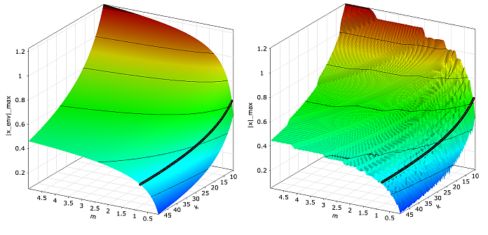
The constraint condition is indicated in the figure by the function w = 8 1/s. If the maximum amplitude is obtained by a time discretization of Equation 3–4 using a coarse time interval, the resulting objective function may contain local oscillations, which may be interpreted as solver noise. In order to demonstrate the behavior of the different optimizers in the presence of small solver noise, a time step of 0.1 seconds is chosen, which leads to a slightly noisy objective function shown additionally in Figure 3.3: Objective Function of the Damped Oscillator.