Response surface methods replace the model responses by mathematical surrogate functions. On this base, the optimization problem is solved using the approximation model instead of time consuming solver calls. The classical procedure uses a Design of Experiments scheme which is evaluated by the solver. Based on these designs often polynomial functions are used for the approximation (Myers and Montgomery 2002). However, the polynomial degree does often not represent the nonlinearity of the solver model and a low quality of the approximation leads often to unusable design suggestions. For this reason it is not recommended to use global polynomial response surface methods only to search for an optimal design.

Figure 3.6: Global Polynomial Approximation

Global polynomial approximation of the maximum amplitude (left, = 98%) and the damped eigen-frequency (right, = 96%) of the optimized oscillator using a quadratic basis and a full factorial design scheme.

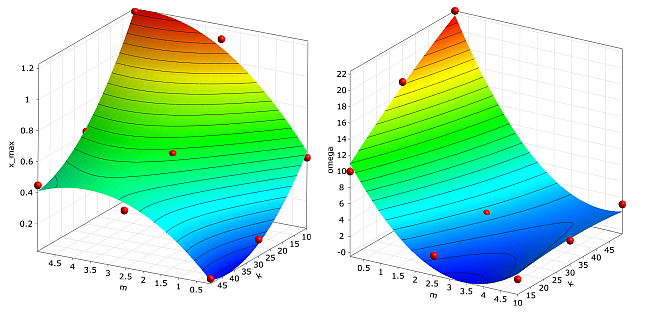
In order to demonstrate the weakness of global polynomial response surface approximation in combination with classical DoE schemes, the maximum amplitude and the damped eigen-frequency of the damped oscillator are approximated by a quadratic polynomial. Support points are generated using a three-level full factorial design. Although the approximation quality is indicated to be very well by means of the adjusted Coefficient of Determination, the optimum found on the approximation (m = 3.31 kg, k = 50.0 N/m) is far away from the true optimum.

Optimization using the Metamodel of Optimal Prognosis

Due to the power of the Metamodel of Optimal Prognosis procedure in finding an optimal variable subspace and an optimal approximation model for each investigated model response, it is strongly recommended to use the MOP approximation for a first optimization step instead of global polynomial models. The Coefficient of Prognosis gives a much more reliable estimate of the approximation quality than the Coefficient of Determination as explained in Coefficient of Prognosis. If the quality of a certain model response, which is used in the objective or constraint functions, is low, the optimization procedure may not find a useful optimized design. In order to check the quality of the optimal design found on the MOP, optiSLang provides a verification of the best design where the solver outputs and the true objective and constraint values are calculated by a single solver call. Often the best design found by the MOP based optimization is better than the best design of the preceding sensitivity analysis. If this is the case, this design could be used as a start design for a further local search.

In the presence of many constraint conditions often the MOP based best design violates one or more of these conditions if the approximation quality is not perfect. This problem can be solved by adjusting the limits of the corresponding constraint conditions in order to push the optimizer running on the approximation back to the feasible region. After each adjustment of the constraint conditions the best design should be verified to check for a possible fulfillment of the critical constraints.

Since the solver noise is smoothed by the MOP approximation, this procedure is more stable than the gradient-based methods. Furthermore, non-convex optimization problems can be solved by using global optimizers such as evolutionary algorithms (EA) on the approximation function. Nevertheless, generally the MOP uses uniformly distributed designs for the approximation model, which may lead to a insufficient local approximation quality around the optimum. Therefore, optimization using global approximation models should be understood as a low-cost pre-optimization step.

In order to demonstrate the benefit of an optimization on the MOP approximation, the damped oscillator is investigated by building the MOP with 100 Latin Hypercube samples. The approximation functions of the MOP are shown in Figure 3.7: Metamodel of Optimal Prognosis.

Figure 3.7: Metamodel of Optimal Prognosis

Approximation of the maximum amplitude (left, CoP = 99%) and of the damped eigen-frequency (right, CoP = 98%) by using the Metamodel of Optimal Prognosis with 100 Latin Hypercube samples

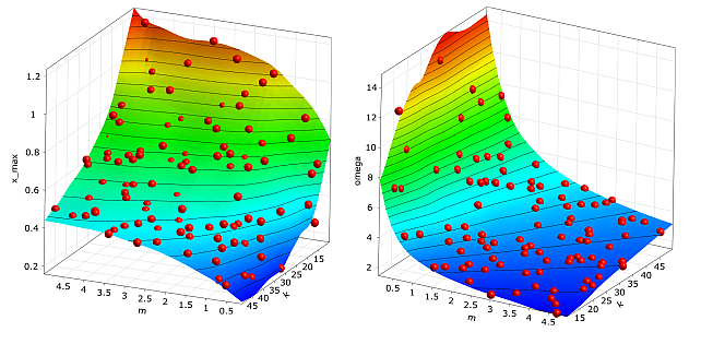
The figure indicates an excellent approximation quality in terms of the Coefficient of Prognosis. By using the MOP approximation functions the optimum is determined very close to the true optimum (m = 0.77 kg, k = 50.0 N/m). The approximated damped eigen-frequency at the obtained optimum is ω = 8.00 1/s, but the real eigen-frequency verified by the solver is ω = 8.04 1/s, which means that the constraint condition is slightly violated. In this case a reduction of the maximum allowed eigen-frequency would force the optimizer to stay in the feasible region.

Adaptive Response Surface Method

In order to improve the approximation quality around the optimum, adaptive meth- ods are very efficient. optiSLang provides a polynomial based local Adaptive Response Surface Method (ARSM). The ARSM procedure starts at a single start design, and an initial Design of Experiments (DoE) scheme is built having the start design as center point. For linear or quadratic polynomial models the corresponding D-optimal design schemes are preferred as DoE schemes. Based on the approximation of the model responses the optimal design is searched within the parameter bounds of the DoE scheme. In the next iteration step a new DoE scheme is built around this optimal design. Depending on the distance between the optimal designs of the current and previous iteration steps, the DoE scheme is moved, shrunken or expanded. This procedure is shown in principle in Figure 3.8. Further details about the adaptation procedure can be found in (Etman et al. 1996) and (Stander and Graig 2002).

Figure 3.8: Adaptation of the Polynomial Approximation Scheme Inside the Adaptive Response Surface Method

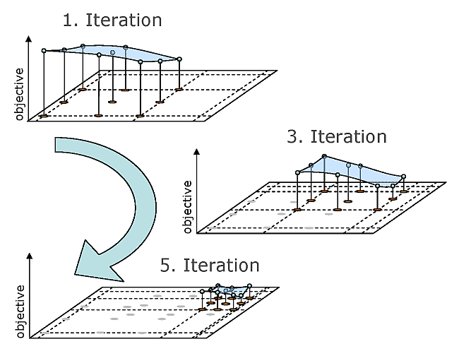
The ARSM algorithm converges if the DoE is shrunken to a minimum size or if the change of the optimal design position and its objective value between two iteration steps is below a specified tolerance. Since the DoE scheme uses 50% more designs than needed for the polynomial approximation, the solver noise is smoothed and few failed designs are not problematic for the optimizer. Due to its efficiency for up to 20 variables and its robustness against solver noise, the ARSM is the method of choice for low dimensional single-objective optimization problems. It is recommended to use the optimal design of a preceding sensitivity analysis as start design for the ARSM. For a strongly localized search the start range of the initial DoE scheme should be reduced.

In Figure 3.9: Convergence of the Adaptive Response Surface Method, the convergence of the ARSM optimizer is shown for the oscilla- tor problem by analyzing the noisy objective function.

Figure 3.9: Convergence of the Adaptive Response Surface Method

Convergence of the Adaptive Response Surface Method for the damped oscillator by using the noisy objective function: designs used for the adaptation (left) and modification of the local DoE bounds during the iteration (right).

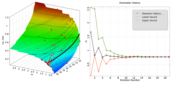
By using a start range of 50% of the design space and a linear polynomial basis, the optimizer runs within a few iteration steps in the region of the true optimum. After 20 iteration steps the algorithm converges at m = 0.77 kg, k = 49.3 N/m, where the constraint condition is fulfilled. This example clarifies that the ARSM optimizer shows a stable convergence behavior for noisy model responses in contrast to the gradient based methods.