


Gradient-based optimization methods use local derivatives of the objective function to find the next local optimum. The minimum of a convex function can be determined by searching for the point, where the first derivative is equal to zero as shown in Figure 3.4: Iterative Search of a Gradient-Based Method Using a Quadratic Approximation of the Objective Function.
Figure 3.4: Iterative Search of a Gradient-Based Method Using a Quadratic Approximation of the Objective Function
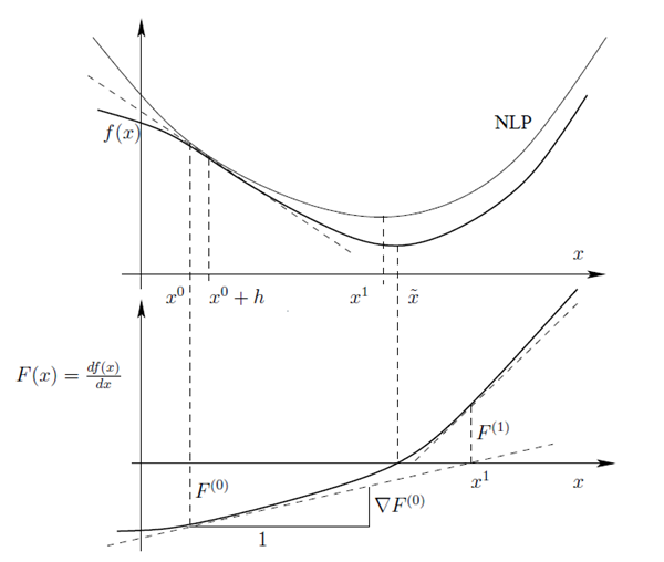
If the second derivatives is known, the objective function can be approximated by a second order Taylor series. This procedure is called Nonlinear Programming (NLP). Optimization methods using first and second order derivatives are known as Newton methods (Kelley 1999). If the CAE solver is treated as black box, the derivatives have to be calculated by numerical estimates. Since second order derivatives would require a large number of solver calls, full Newton methods are not applicable for complex optimization problems. For this reason quasi Newton methods have been developed, where the second order derivatives are approximated from the first order derivatives of previous iteration steps. Gradient-based methods distinguish each other mainly in the way how the second order derivatives are estimated and how additional constraint equations are considered. A good overview over different methods in given in (Kelley 1999).
In optiSLang the NLPQL approach (Nonlinear Programming by Quadratic Lagrangian) is preferred (Schittkowski 1986). First-order derivatives of the objective and constraint functions are estimated from central differences or by one-sided numerical derivatives using a specified differentiation interval. The NLPQL approach features efficient constraint handling using quadratic Lagrangian. Starting from a given start point, the method searches for the next local optimum and converges if the estimated gradients are below a specified tolerance. Since it is a local optimization method, it is recommended to use the best design of a global sensitivity analysis as start point in order to find the global optimum. The NLPQL is very efficient in low dimensions with up to 20 design variables. For higher dimensional problems the computation of the numerical derivatives becomes more and more expensive and other methods are more efficient. In the presence of noisy model responses the differentiation interval plays a crucial role. If its taken too small, the estimated gradient is distorted heavily by the solver noise and the NLPQL runs into a wrong direction. If the solver noise is not dominating the functional trend an increased differentiation interval could lead to a good convergence of the optimization procedure.
|
|
|
Convergence of the NLPQL optimizer for the oscillator optimization problem by using the smooth objective function based on the envelope estimate (left) and by using the noisy objective function from the time discretization (right). |
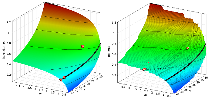
In Figure 3.5: Convergence of the NLPQL Optimizer, the convergence of the NLPQL approach is shown for the optimization of the damped oscillator: in the first investigation, the smooth objective function obtained from the envelope curve estimate is considered. In this case the optimizer converges in three iteration steps to the true optimum (m = 0.78 kg, k = 50.0 N/m). If the noisy objective function is investigated with a relatively small differentiation interval (1% of the design space) the optimizer runs into the wrong direction and will not converge to the true optimum. Nevertheless, by increasing the differentiation interval the convergence to the true optimum can be achieved for this example.