


Population based optimization methods imitate natural processes like biological evolution or swarm intelligence. Based on the principle ’survival of the fittest’ a population of artificial individuals searches the design space of possible solutions in order to find a better approximation for the solution of the optimization problem.
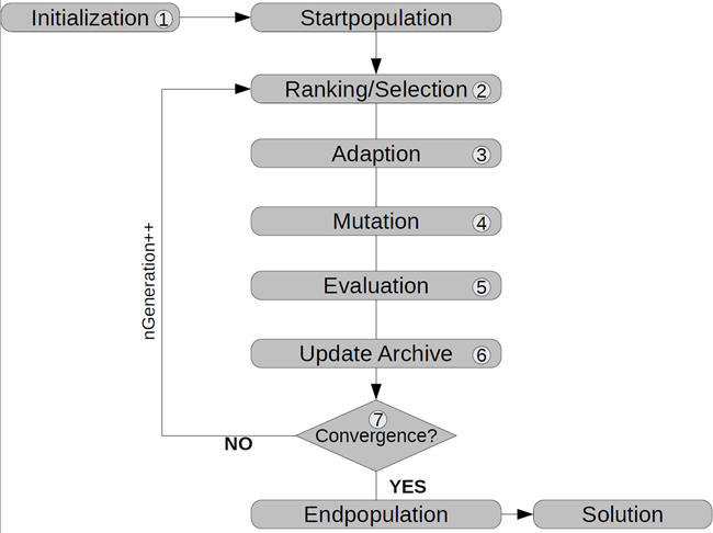
All kinds of population based algorithms are following a particular flow. It starts with a random initialization (see Figure 3.10: General Flowchart of Population Based Optimization Algorithms, step 1) of a population containing µ individuals representing possible solutions to the given optimization problem.
After initialization the actual iteration loop starts, where every loop represents a generation. To create a new generation the fittest designs will be selected (step 2). The adaption referred to step 3 can be done in different ways, e.g. crossover or swarm movement. Mutation (step 4) can be applied afterwards. All individuals are evaluated (step 5) by assigning them a fitness value based on the objective value and possible constraint violations. Thus a high fitness score means a good accommodation to the problem and corresponds with a small objective value. After evaluating each design the archive, which keeps good solutions, will be updated for the next selection step (step 6). The generation counter is increased and the iteration continues until a stopping criterion is fulfilled (step 7).
The efficiency of population based methods can be significantly improved by choosing a suitable start population. If the optimization is performed after an initial sensitivity analysis, it is strongly recommended to use the best designs of the sensitivity analysis as start population. In order to keep the global character of the optimization it is useful to select designs covering a certain range of the design space.
The usage of population based algorithms is recommended in a wide range of applications. They are often the last resort for solving mathematically ill conditioned problems since their performance may be still good in case of a high number of design variables or a high amount of failed designs. Nevertheless, the convergence behavior may be slower compared to other optimization methods. The use of population based algorithms is recommended in all cases where gradient based optimization or response surface approximation fails, in case of a high number of variables or constraints, in case of discrete or binary design variables, in case of discrete responses or if the user is unaware about the optimization problem.
Evolutionary Algorithms
Evolutionary algorithms (EA) are stochastic search methods that mimic processes of natural biological evolution. Many EA variants have been implemented over the past decades, based on the three main classes: genetic algorithms (GA) (Holland 1975), evolution strategies (ES) (Rechenberg 1964) and evolutionary programming (EP) (Fogel et al. 1966). These algorithms have been originally developed to solve optimization problems where no gradient information is available, like binary or discrete search spaces, although they can also be applied to problems with continuous variables. Within optiSLang there is a flexible implementation of genetic algorithms and evolutionary strategies available which allows to scale between pure (strong) GA and pure (strong) ES.
After the random or manual initialization of a population containing µ individ- uals the actual iteration loop starts, where every loop represents a generation g. Selection determines λ individuals for reproduction based on its fitness or ranking. Different stochastic selection operators are provided in order to adjust the selection pressure. Parent selection sets the direction of the stochastic search process. Variation is introduced by applying crossover and mutation operators to the selected individuals. These new individuals are called newborns or offspring. Finally the resulting offspring individuals are evaluated and a new population of µ individuals is formed using a replacement scheme.
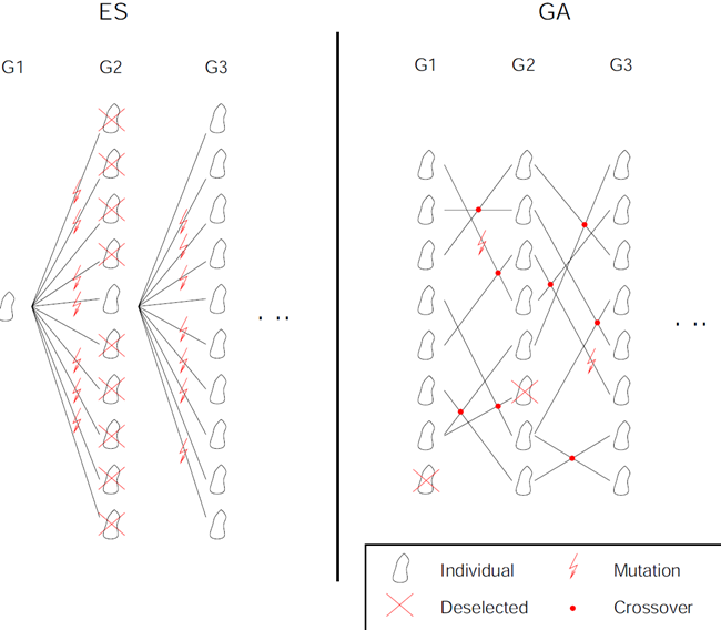
The main difference between the two main variants, genetic algorithms (GA) and evolution strategies (ES), is the way variation is introduced to the population. Recombination of genes using crossover operators represents the main variation within genetic algorithms, while for evolution strategies (adaptive) mutation introduces variation to the population (see Figure 3.11: Evolution Strategies Versus Genetic Algorithms).
The selection of individuals for reproduction is based on random selection methods and requires an assignment of fitness values. A rank-based fitness assignment is used to overcome the scaling problem of the proportional fitness assignment. Due to the random selection and the fitness ranking, the probability of selecting a design with low fitness is low. However, this is not impossible, so also a weak design could be used for the generation of offspring.
The crossover operator is a method of recombination where two parent individuals produce two offspring by sharing information between chromosomes. The intention is to obtain individuals with better characteristics (exploitation) and to maintain the diversity of the population (exploration). Crossover is regarded as the main search operator in genetic algorithms.
Mutation introduces random variation to the genes of the offspring chromosome. Each gene is selected for mutation with a specified probability or mutation rate respectively. The real-valued mutation is based on a normal distribution function for each gene with the value of the gene as its mean value. Mutation is the main search operator for evolutionary strategies (ES) but can also be applied after recombination (see Figure 3.10: General Flowchart of Population Based Optimization Algorithms). The mutation rate and the standard deviation defined in relation to the variable range are the control parameters of the mutation which can stay constant or get modified during the run of the algorithm. optiSLang provides constant and adaptive mutation procedures. Further details can be found in (Bäck 1996) and (Riedel et al. 2005).
The final operator, the archive update scheme, specifies how the population of the next generation is formed out of individuals of the current population (µ) and the generated offspring individuals (λ). The µ best individuals for the next generation are selected from a selection pool. Different strategies of constituting the selection pool are available by adjusting the size of the archive (α). The (µ, λ)-strategy with empty archive leads to a complete replacement of the population at every generation step with a maximum life span of an individual of only one generation. This method is used for classic genetic algorithms. The (µ + λ)-strategy prevents archive individuals from being replaced by offspring with worse fitness. This strategy is recommended for use with evolution strategies. The (α(µ) + λ)-strategy allows the adjustment of the archive update scheme between the two extreme cases.
optiSLang provides a parameter-free constraint handling method taking into account all individuals of the population, which are compared regarding their objective values and constraint violations. The infeasible solutions are ranked according their constraint violations and their fitness is modified by adding the fitness of the worst feasible solution to the rank value. This procedure does not require additional penalty parameters. Furthermore it can handle multiple constraints without scaling of constraint values. Even if all individuals are violating constraints, the method can guide the search towards a feasible region of the constraint space.
In optiSLang a predefined global and local search is available for the evolutionary algorithms. The global search starts with a random or manually selected start population and is suitable to detect new possible solutions in the whole design space. The local search tries to improve a single design without discovering new regions. In Figure 3.12: Convergence of the Evolutionary Algorithm, both search strategies are compared.
|
|
|
Convergence of the evolutionary algorithm with global search (left) and local search (right) for the damped oscillator with noisy objective function. |
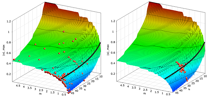
The figure indicates, that the global search, which starts with a random start population, generates designs in the whole design space while the designs generated with the local search method stay close to the start design. Due to the applied random search strategies in evolutionary algorithms the optimizer may not converge very close to the global optimum always. For example, the optimum found for the damped oscillator by using the global search (m = 0.81 kg, k = 50.0 N/m) is not as good as the results of the ARSM optimizer. For this reason it is often useful to use the evolutionary algorithms to detect the region of the global optimum and do further improvements with other optimization methods.
Particle Swarm Optimization
Particle Swarm Optimization (PSO) is a nature-inspired optimization method developed by (Kennedy and Eberhart 1995) that imitates the social behavior of a swarm. Information about preferred positions will be transmitted to other individuals of the swarm such that they move into directions of previous optimal positions. In nature an individual can be represented by a bird, bee or fish. An overview of modifications and improvements of this class of algorithms can be found e.g. in (Engelbrecht 2005) and (Poli et al. 2007).
|
|
|
Update of a particle position |
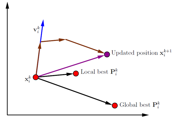


PSO starts with initializing a population of size µ where each individual represents a possible solution of the optimization problem. Swarm intelligence is influenced by two main components representing the personal and global behavior. This means that each individual remembers its personal best solution and will also be influenced by the best solution of the swarm. Each individual will change its position xi into the direction of its personal best found position Pi and the global best found position Pg .
 | (3–6) |
There are three important parameters that influence the speed and spread of the swarm. The inertia weight w is a scaling factor for the velocity of the previous iteration step k. The personal acceleration coefficient cp is a scaling factor for the second term, which is also called cognitive component. The third term, called social component, is scaled by the global acceleration coefficient cg . R1 and R2 are two vectors of random numbers uniformly chosen from [0, 1].
The choice of suitable coefficients cp , cg and w is very important for the convergence behavior of the PSO. optiSLang provides two predefined search strategies with default values for each coefficient. A local search strategy is recommended if the user has preliminary information about the optimization space and has already found a pre-optimized design. In this case the swarm movement is slower and less intensive throughout all generations. In a predefined global search strategy the swarm movement is very intensive at the beginning and will be damped throughout the optimization process by decreasing the weights of the previous velocity and the cognitive component and increasing the weight of the social component. In that way a global exploration is reached in the first iterations and exploitation is possible in last iterations.
To allow a more sophisticated search, optiSLang enables the same mutation methods that are available for evolutionary algorithms. For executing a classical PSO search one has to deselect the mutation operator. The global best solution is recorded in the archive and is updated at the end of each iteration step. In the presence of constraint conditions the global best solution is found by taking the feasible solution with minimal objective value. If there are only infeasible solutions in the first population the global best will taken as the individual with least constraint violations.
The PSO works similarly to the evolutionary algorithms for optimization problems with a large amount of failed designs. It is less efficient compared to evolutionary algorithms if discrete design variables and many constraint conditions are investigated. For optimization tasks with continuous design variables the PSO converges generally very close to the global optimum. Similar to evolutionary algorithms, the choice of a qualified start population e.g. from sensitivity analysis may significantly improve the efficiency of the algorithm.
Stochastic Design Improvement
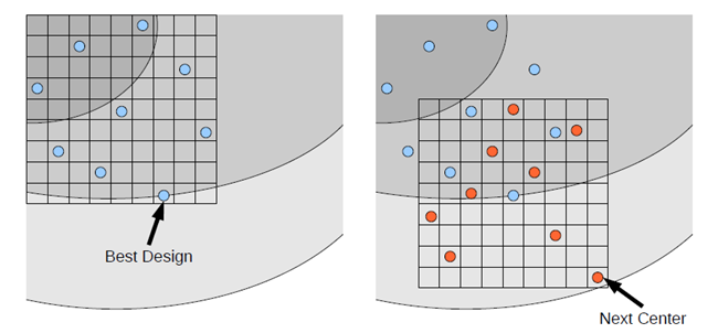
Stochastic Design Improvement (SDI) is a local, single-objective optimization procedure that improves a proposed design by using a simple stochastic approach without having extensive knowledge about potential relationships in design space. Based on an initial start design, a start population of size µ is generated by an uniformly distributed Latin Hypercube Sampling within a given range. In each iteration step, the best design is taken as new center point for the sampling of the next iteration as shown in Figure 3.14: Stochastic Design Improvement. The ranges of the sampling scheme are adapted in each iteration step. Depending on the optimization problem the whole population might move into a better region and achieve an improvement in each step. All individuals of one iteration will be compared concerning objective and constraints by using the parameter-free constraint handling method applied in the evolutionary algorithms. The algorithm converges if either a maximum number of iterations was reached, if a specified improvement with respect to the initial design was reached (gained improvement) or if a specified deterioration of the performance between two iteration steps was observed.
|
|
|
Update scheme of the Stochastic Design Improvement approach by generating a random sampling around the best design of a previous iteration. |
Due to its pure stochastic approach the SDI is very robust and works for a high amount of failed designs, discrete and continuous parameters, and a high number of design variables and constraint conditions. Nevertheless, it was designed to improve an initial design but not to find global optimal solutions. For this reason its efficiency may be significantly lower compared to evolutionary algorithms and Particle Swarm Optimization.