


| Analysis Type | Cyclic Symmetry |
| Features Demonstrated | Forced Response Add-on, static structural system, harmonic response system, external data pressure |
| Licenses Required | Ansys Mechanical Enterprise/Enterprise Solver/Enterprise PrepPost |
| Help Resources | Forced Response Add-on |
| Tutorial Files | Mistuning.zip |
This tutorial guides you through the following topics:
The Forced Response Add-on provides a comprehensive way of investigating the aeromechanics, and ultimately, the reliability of turbomachinery blade rows. The Forced Response application is an add-on to the Ansys Mechanical user interface that enables you to use cyclic modeling.
Data files for this tutorial can be found here on the Ansys customer site. The files you need are:
Blade.pmbd - geometry input file
Kmist.csv - mistuning input file
WS01_CFX_Pressure.csv - external data of pressure input file
Begin the project in Workbench.
Drag a Static Structural system onto the Project Schematic.
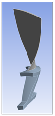
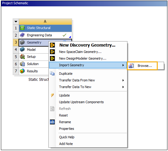
Right-click the Geometry cell, and under Import Geometry, insert Blade.pmbd from the input files.
Blade.pmbd is an imported geometry of a single sector called the base sector. Cyclic symmetry analyses require the modeling of this type of geometry. A proper base sector represents one part of a pattern that, if repeated n times in cylindrical coordinate space, yields the complete model.
Right-click the Model cell and select Edit to open Mechanical.
Continue the configuration in Mechanical.
Right-click the Model in the Outline tree and insert a Virtual Topology. Keep the default options.
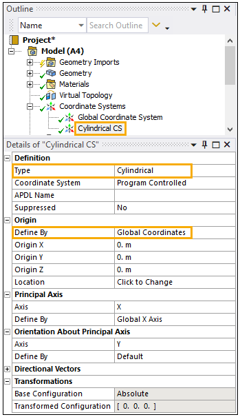
To define the blade symmetry object, a cylindrical coordinate system is required. Insert it by right-clicking Coordinate Systems and selecting Coordinate System. In the Details panel, set the following properties:
Type: Cylindrical
Define By: Global Coordinates
Rename the Coordinate System to Cylindrical CS to identify it.
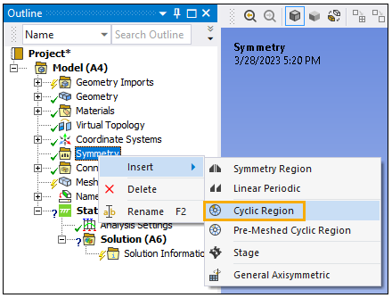
Right-click the Model and insert a Symmetry object. Then right-click the Symmetry object and insert a Cyclic Region. Assign the following Cyclic Region properties in the Details panel:
Scoping Method: Named Selection
Low Selection: CYCSYMMFACE2
High Selection: CYCSYMMFACE1
Coordinate System: Cylindrical CS

Create the mesh definition in Mechanical.
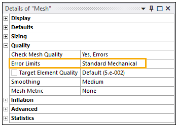
Click Mesh in the Outline tree, then navigate to its Details panel. In the Quality section, change the Error Limits to Standard Mechanical.
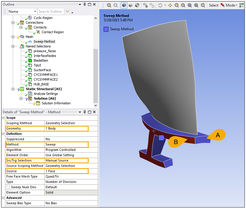
Insert a Method by right-clicking the Mesh in the Outline tree. Set the following Method properties in the Details panel:
Geometry: The component or solid body (A in the image below)
Method: Sweep
Src/Trg Selection: Manual Source
Source: 1 face (B)
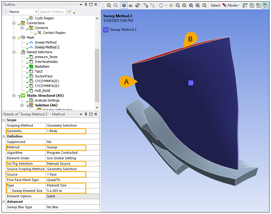
Insert another Method under the Mesh. Set it to the following properties:
Geometry: The component or blade body (A in the image below)
Method: Sweep
Src/Trg Selection: Manual Source
Source: The top face of the blade (B)
Type: Element Size
Sweep Element Size: 0.005m
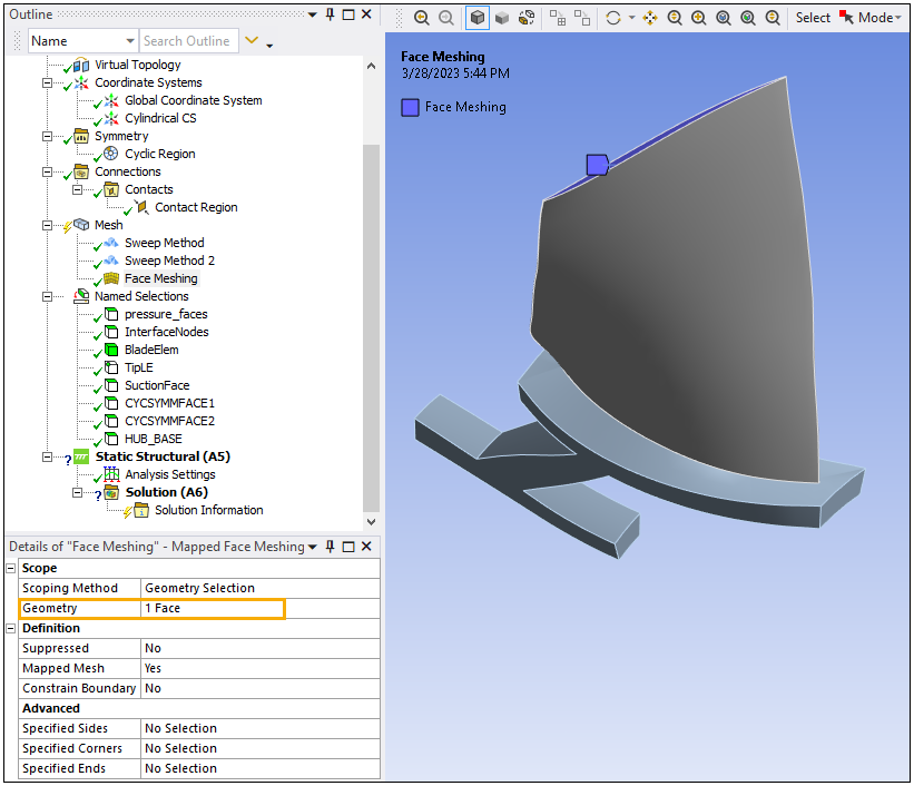
Insert a Face Meshing under the Mesh and scope its Geometry to the top face of the blade.
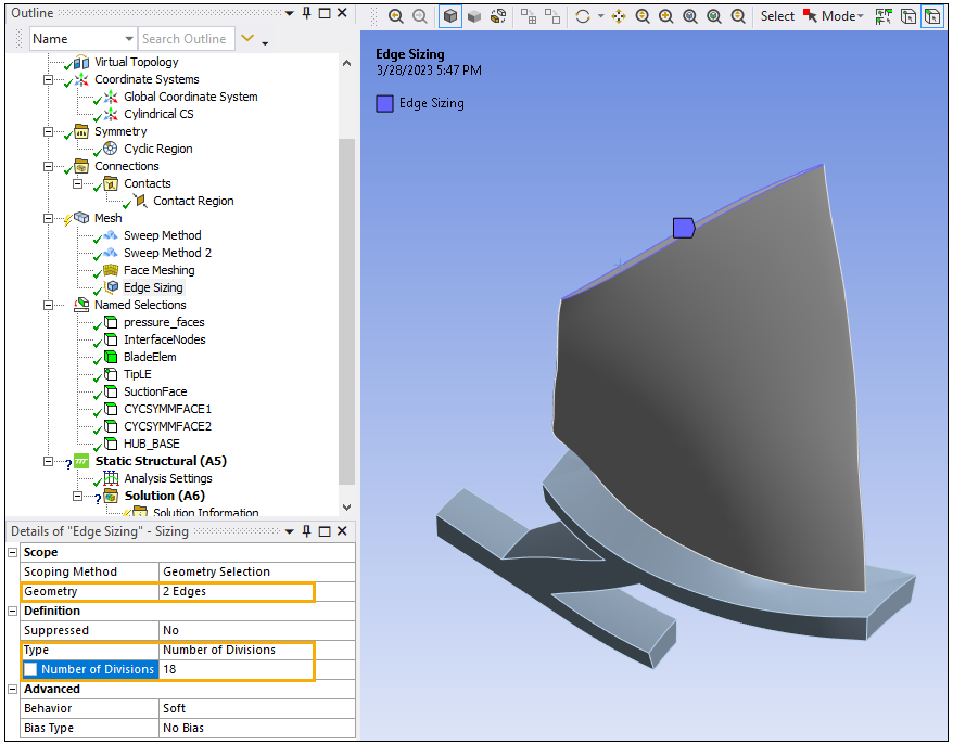
Insert a Sizing under the Mesh and configure its properties with:
Geometry: The two edges of the top surface of the edge
Type: Number of Divisions
Number of Divisions: 18
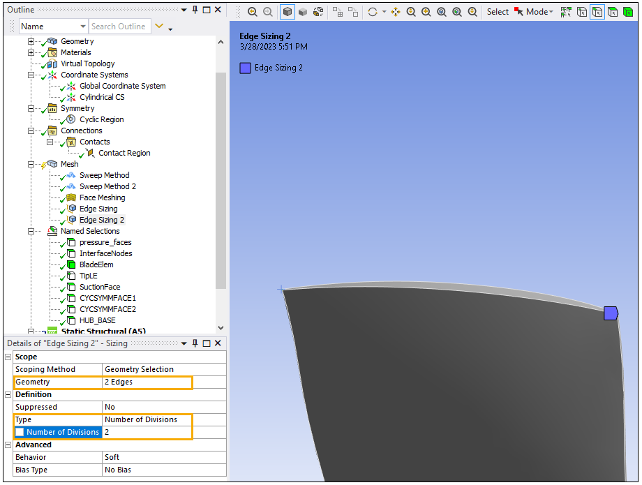
Similarly, apply another Sizing to the Mesh and set the following properties:
Geometry: The two small top edges of the blade (A and B, below)
Type: Number of Divisions
Number of Divisions: 2
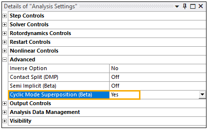
Click Analysis Settings in the Outline tree. In its Details panel, set the Cyclic Mode Superposition (Beta) field to Yes.
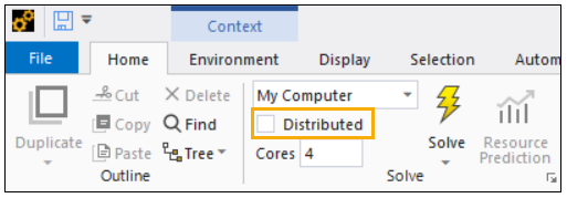
In the Home tab's toolbar, deselect the Distributed check box.
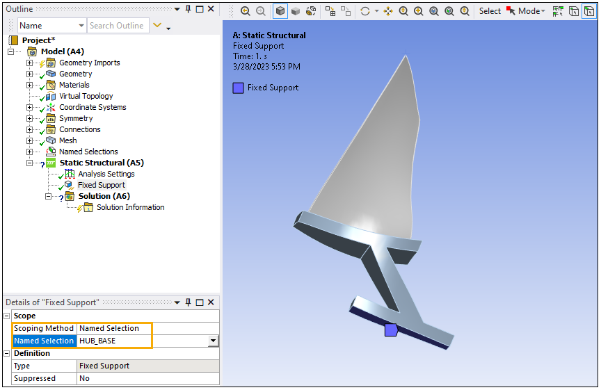
Insert a Fixed Support to the Static Structural system. Set its properties as follows:
Scoping Method: Named Selection
Named Selection: HUB_BASE
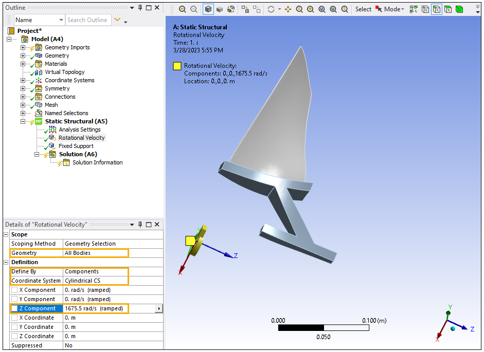
Insert a Rotational Velocity to the Static Structural system. Set the following properties:
Geometry: All Bodies
Define By: Components
Coordinate Systems: Cylindrical CS
Z Component: 1675.5 radians per second
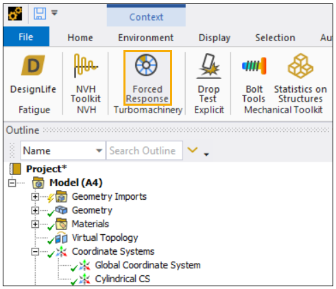
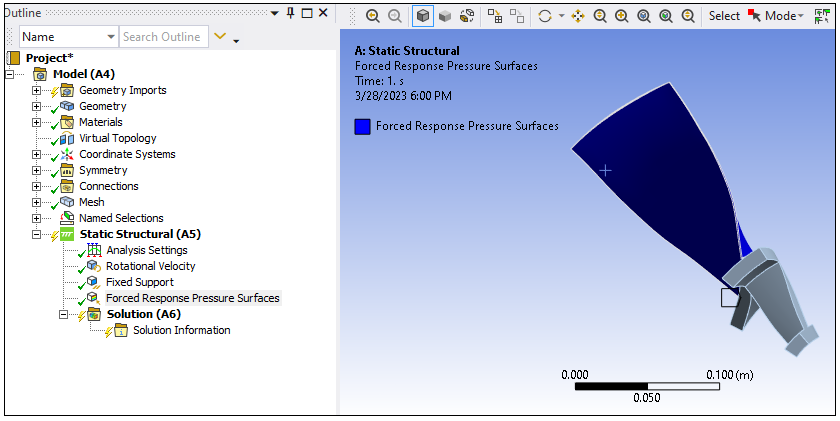
Go to the Add-ons tab, and click the Forced Response icon to turn it on. Note that the new tab for the Forced Response capabilities appears in the ribbon.
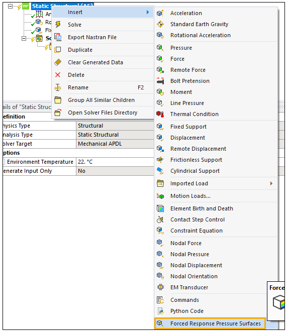
Insert a Forced Response Pressure Surfaces object to the Static Structural system. In the Details panel, scope its Geometry to the five faces of the blade.
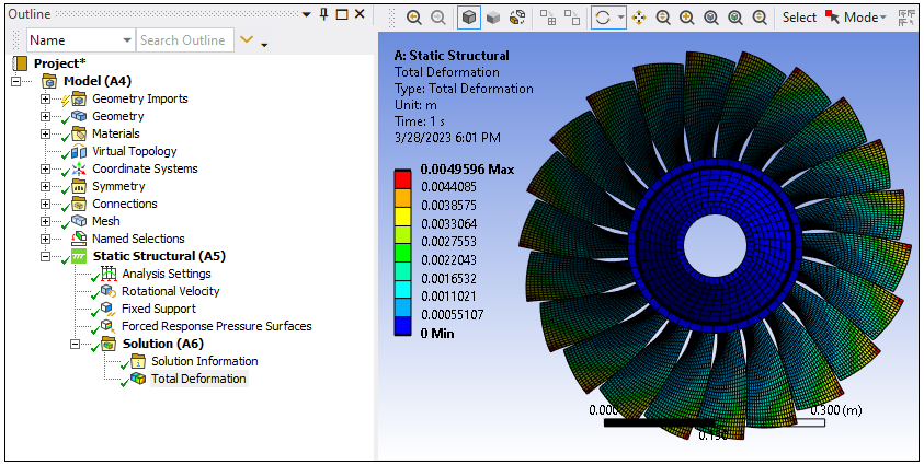
Right-click the Solution and insert a Total Deformation for the result. Solve the model and evaluate that the results are correct.
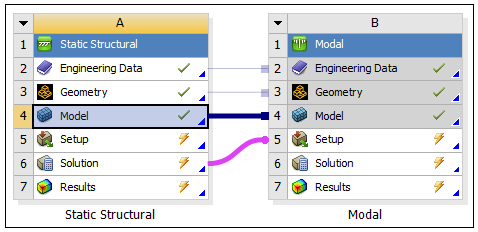
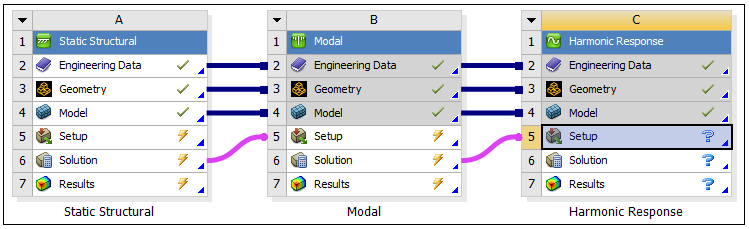
Go back to the Project Schematic in Workbench and drag a Modal system onto the Static Structural. This connects the Solution cell of the Static Structural system to the Setup cell of the Modal system.
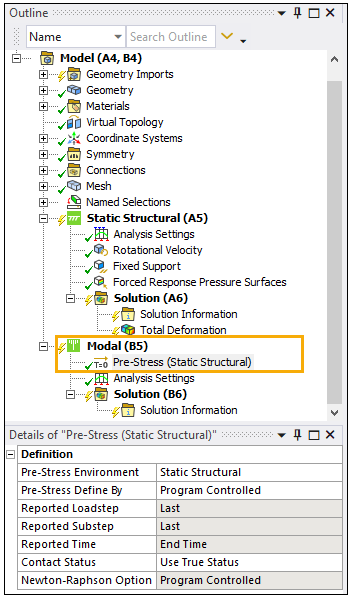
Return to Mechanical to set up the Modal analysis. Note that the Modal system is Pre-Stressed with the Static Structural system.
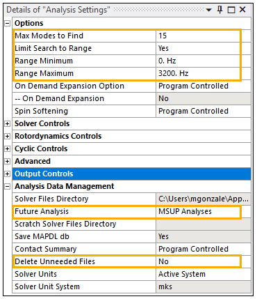
Select the Analysis Settings and set the following properties in the Details panel:
Under Options:
Max Nodes to Find: 15
Limit Search: Yes
Range Minimum: 0 Hz
Range Maximum: 3200 Hz
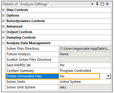
Under Analysis Data Management:
Future Analysis: MSUP Analyses
Delete Unneeded Files: No (otherwise, many required files for postprocessing Forced Response results will be deleted)
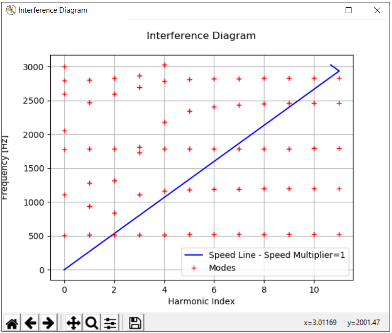
Solve the Modal system. Then insert an Interference Diagram to the Solution. The Rotation Speed is read from the Static Structural analysis and can be edited. One or more engine orders may be plotted by setting values separated with commas (','). Only positive values are accepted. Once that is done, click the Apply button to display the Campbell Diagram.
Note: The Campbell Diagram does not always guarantee true resonance. Instead, it suggests that resonance will occur whenever the natural frequency of the block matches the excitation frequency. Due to the cyclic nature of the structure, the mode shape may not match the engine order's excitation shape coming out of the nozzles for the suggested critical speed of the Campbell Diagram. Hence, the SAFE or Interference Diagram, which relates the mode shapes with speed and natural frequency, will predict the true resonance and is used by industries for reliable design.
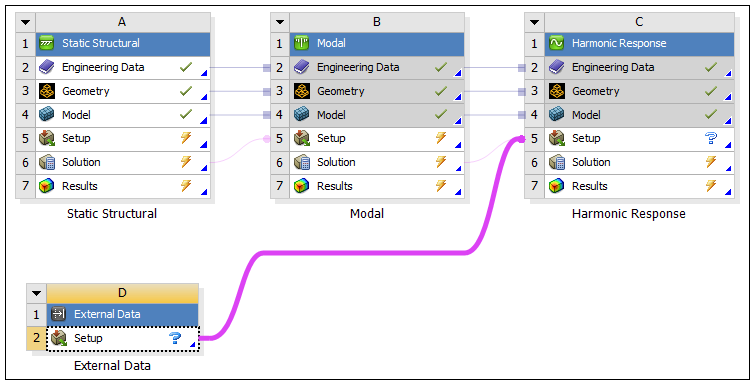
Go back to the Project Schematic in Workbench and insert a Harmonic Response system onto the Modal system, which connects the Solution cell of Modal to the Setup cell of Harmonic Response.
Return to Mechanical to set up the Harmonic Response analysis.
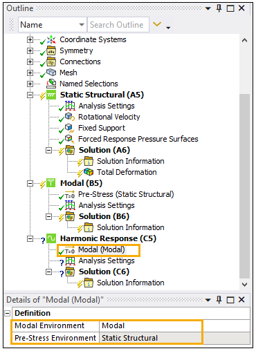
Ensure that the Harmonic Response system's Modal properties are set to the following:
Modal Environment: Modal
Pre-Stress Environment: Static Structural
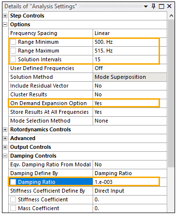
Select the Analysis Settings and set the following properties:
Range Minimum: 500 Hz
Range Maximum: 515 Hz
Solution Intervals: 15
On Demand Expansion Option: Yes
Under Damping Controls:
Damping Ratio: 0.001
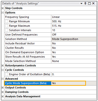
Under Analysis Data Management:
Delete Unneeded Files: No
Under Advanced:
Cyclic Mode Superposition (Beta): Yes
In this tutorial, you will apply pressure using the External Data system.
Go to the Project Schematic in Workbench.
Drag External Data from Component Systems onto the schematic to create a stand alone system. Then drag its Setup cell onto the Harmonic Response system's Setup cell to connect them.
Import Engineering Data in Workbench.
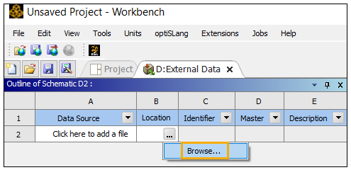
Double-click the Setup cell of the External Data system to open the External Data tab.
From the Location column, Browse to the WS01_CFX_Pressure.csv input file.
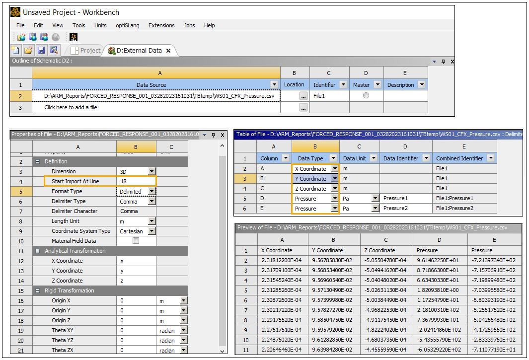
Click the imported file's name in the Data Source column to view its contents. Configure its data type as follows:
Under Properties of File:
Start Import at Line: 18
Under Table of Files:
Column B:
Row 2: X Coordinate
Row 3: Y Coordinate
Row 4: Z Coordinate
Row 5: Pressure
Row 6: Pressure
Return to the Project tab and Update the Setup cell of External Data.
Update the Setup cell of the Harmonic Response system.
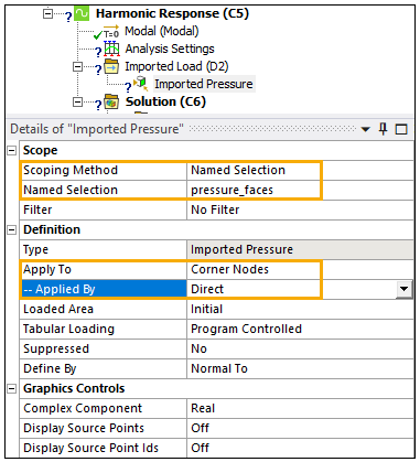
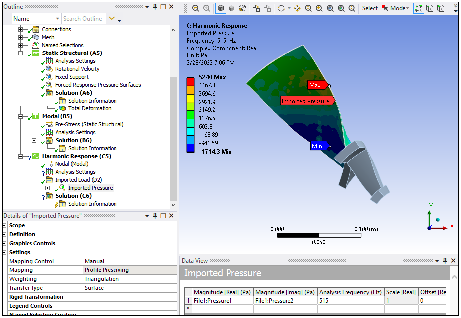
Return to Mechanical and note that the Imported Load folder appears under Harmonic Response. Right-click the folder and insert Pressure. Set the Pressure properties as follows:
Scoping Method: Named Selection
Named Selection: pressure_faces
Applied To: Corner Nodes
Applied By: Direct
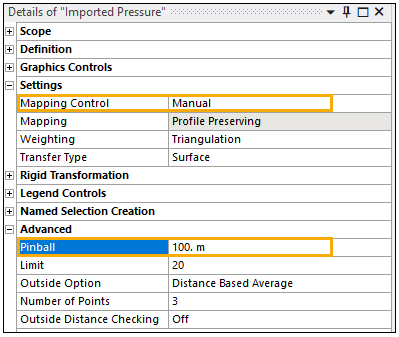
Under Settings:
Mapping Control: Manual
Under Advanced:
Pinball: 100 m
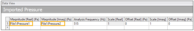
In the Data View, set the following Imported Pressure magnitudes:
Real: Pressure1
Imaginary: Pressure2
Right-click the Imported Pressure object in the Outline tree and select Import Load to map the pressure on your blade surfaces.
Small mistuning effects (on the order of a few percent) may be included in the analysis by introducing blade-to-blade variations in the stiffness (frequency) of each blade. The Mistuning object takes tuned response and adds the mistuning effects of each blade in a cyclic analysis. Variation of blade stiffnesses should not be more than 10%. For more information on the Mistuning object, see Mistuning Settings in the Mechanical Add-ons Guide.
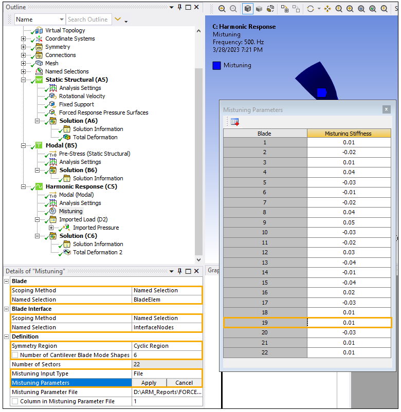
In Mechanical, right-click Harmonic Response and insert a Mistuning object. Set its properties as follows:
Under Blade:
Scoping Method: Named Selection
Named Selection: BladeElem
Under Blade Interface:
Scoping Method: Named Selection
Named Selection: InterfaceNodes
Under Definition:
Symmetry Region: Cyclic Region
Number of Cantilever Blade Mode Shapes: 6
Mistuning Input Type: File
Mistuning Parameter File: Kmist.csv input file
View the Tabular Data to:
Ensure the Mistuning Parameters are populated
Change, as an example, the Blade 19 mistuning stiffness to 0.01
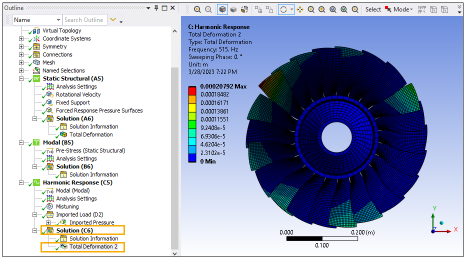
Under Harmonic Response, right-click Solution and insert a Total Deformation.
Solve the Harmonic Response system.
Suppress the Mistuning object and Solve the system again. Note that these Total Deformation results do not account for mistuning.
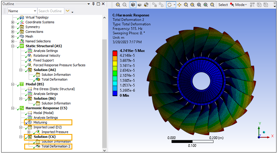
Right-click Solution and insert a Mode Multiplier. In its Details panel, set Frequency [Hz] to 510.5, right-click Mode Multiplier, and select Evaluate All Results to get the result.
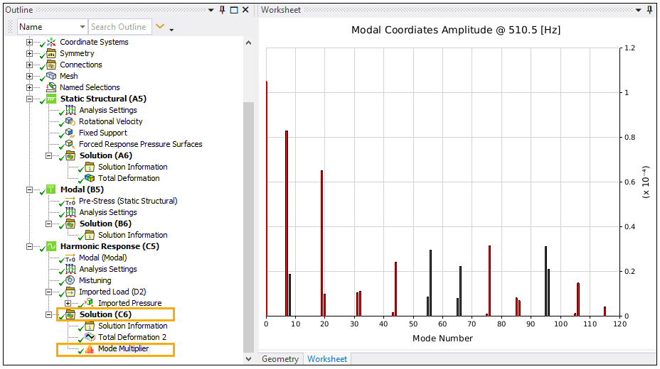
Congratulations! You have completed the tutorial.