


| Analysis Type | Aero coupling |
| Features Demonstrated | Forced Response Add-on |
| Licenses Required | Ansys Mechanical Enterprise/Enterprise Solver/Enterprise PrepPost |
| Help Resources | Chapter 26: Nonlinear Analysis of a Rubber Boot Seal, Forced Response Add-on |
| Tutorial Files | Aerocoupling_addon.zip |
This tutorial guides you through the following topics:
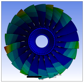
Aerodynamic coupling effects can be included in Forced Response analyses. Aerodynamic coefficients account for vibration-induced pressure fluctuations on the blade surface and contribute to the stiffness and damping of the system. These values can be computed according to the equations for Aerodynamic Coupling in the Theory Reference and are included in cyclic mode-superposition harmonic response analyses using the CYCFREQ,AERO command. The aerodynamic coefficients can be computed directly using a CFD flutter or aerodamping analysis. The aerodynamic coupling coefficients can also be computed using CFD pressures in conjunction with the AEROCOEFF command. For more information on computing and using aerodynamic coefficients, see Aero Coupling.
Important: Refer to this previous tutorial, Turbomachinery Mistuning Analysis using the Forced Response Add-on, before starting this one. This tutorial is a continuation of the that one and you will use that geometry file.
Data files for this tutorial can be found here on the Ansys customer site.
Unsuppress the Mistuning object under the Harmonic Response system. Then proceed with the following steps.
In the Outline tree, insert an additional Coordinate System and set the following properties in the Details panel:
Type: Cylindrical
Define By: Global Coordinates
Origin X: 0
Origin Y: 0
Origin Z: 0
Navigate to the Coordinate System tab and click the Rotate Z action in the toolbar.
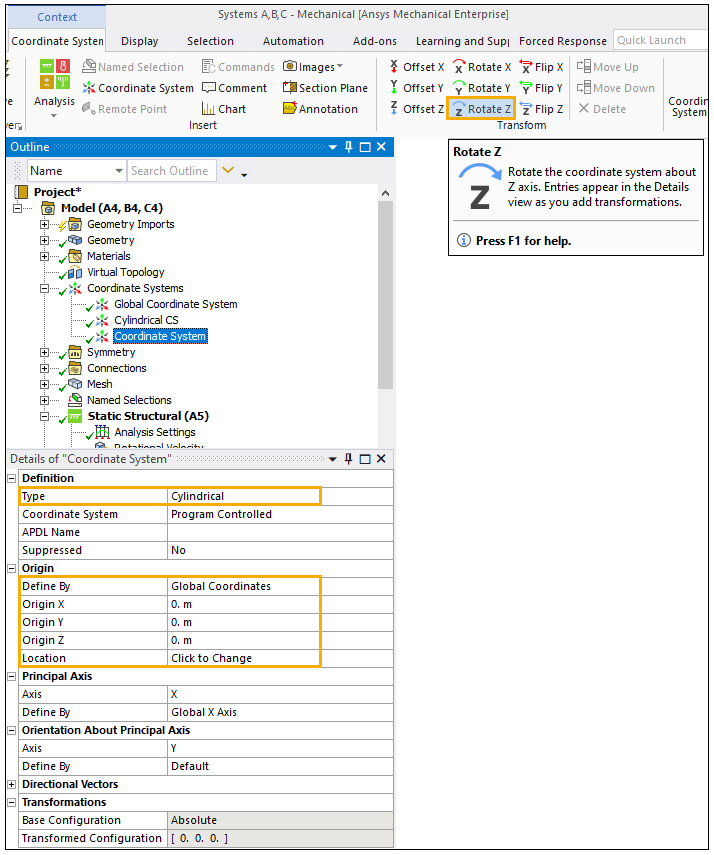
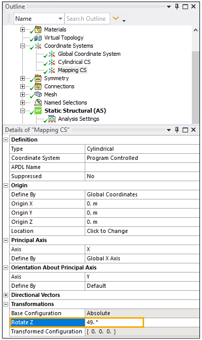
Return to the Details panel and apply a 49° rotation to Rotate Z. Then rename the Coordinate System to Mapping CS.
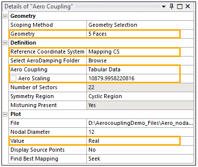
Reference Coordinate System: Mapping CS (created earlier)
Note: The Reference Coordinate System of the Aero Coupling objects must be selected so that the Source Points are aligned with the Geometry. You can check if they are aligned by switching the Display Source Points to Yes. If the Source Points are displayed correctly, that means the Coordinate System definition is correct. Once you finish checking, set the Display Source Points back to No.
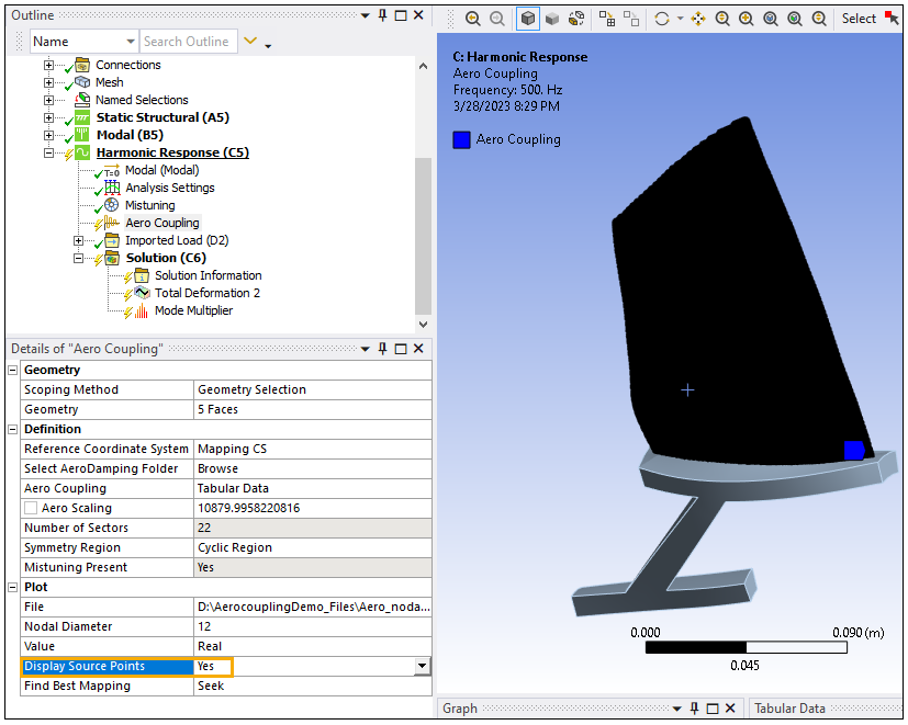
Aero Coupling:
Click Tabular Data
Enter the following Aerodamping Files from the input files and their corresponding Nodal Diameters:
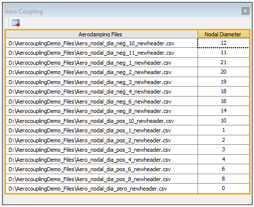
Aero Coupling or aerodamping coupling files can be included if they were generated using CFX.
Check the Tabular Data to ensure that the nodal diameters are associated with the correct files. For more information on nodal diameters, see Modal Cyclic Symmetry Analysis.
Click Apply on Aero Coupling to save the data.
The aero scaling and nodal diameter are read from the files and may be modified.
Aero Scaling: 10879.9958220816
Under Plot:
Value: Real
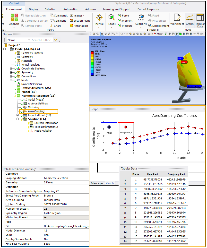
Right-click the Aero Coupling object and select Generate which will take a few seconds to run. Once it has generated, the Real values and AeroDamping Coefficients for each blade will appear in the Graph window.
Right-click the Solution of the Harmonic Response system and select Solve.
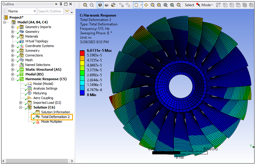
Select the Total Deformation to view the impact of the Aero Coupling object on the result.
Right-click the Solution and insert the Matrices result. Leave the default options so that the Mrom, Krom, and AeroMet matrices are calculated. For each matrix, the real and imaginary values will be displayed or copied. Therefore, the four matrices (real Mrom, imaginary Mrom, real Krom, imaginary Krom) and Aero matrices will be produced by default.
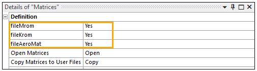
Right-click the Matrices result object and select Evaluate.
After the evaluation, open the matrices in the default editor in .csv format by clicking the Open button. The following .csv files will appear with their corresponding information:
Mrom_Real.csv
Mrom_Imaginary.csv
Krom_Real.csv
Krom_Imaginary.csv
AeroMat_Real.csv
AeroMat_Imaginary.csv
Congratulations! You have completed the tutorial.