


This tutorial demonstrates the use of Interface Delamination feature available in Mechanical by examining the displacement of two 2D parts on a double cantilever beam. This same problem is demonstrated in VM248 in the Ansys Mechanical APDL Verification Manual. The following example is provided to demonstrate the steps to set up and analyze the same model using Mechanical.
| Analysis Type | Interface Delamination |
| Features Demonstrated | Engineering data/materials, static structural analysis, match control, interface delamination |
| Licenses Required | Ansys Mechanical Enterprise/Enterprise Solver/Enterprise PrepPost |
| Help Resources | VM248: Delamination Analysis of Double Cantilever Beam |
| Tutorial Files | 2D_Fracture_Geom.agdb |
This tutorial guides you through the following topics:
- 7.1. Problem Description
- 7.2. Create Static Structural Analysis
- 7.3. Assign Materials
- 7.4. Attach Geometry
- 7.5. Define 2D Behavior
- 7.6. Define Coordinate Systems
- 7.7. Define Mesh Options and Controls
- 7.8. Define Interface Delamination Object
- 7.9. Configure the Analysis Settings
- 7.10. Define Boundary Conditions
- 7.11. Specify Result Objects and Solve
- 7.12. Review the Results
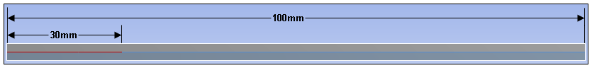
As illustrated below, a two dimensional beam has a length of 100 mm and an initial crack of length of 30 mm at the free end that is subjected to a maximum vertical displacement (Umax) at the top and bottom of the free end nodes. Two vertical displacements, one positive and one negative, are applied to determine the vertical reaction at the end point. The point of fracture is at the vertex of the crack and the interface edges.
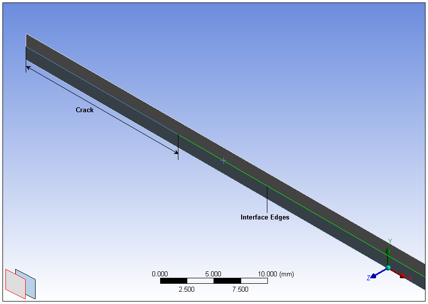
This image illustrates the dimension of the model.
This tutorial also examines how to prepare the necessary materials and mesh controls that work in cooperation with the Interface Delamination feature.
Open Ansys Workbench.
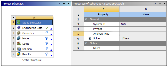
On the Workbench Project page, drag a Static Structural system from the Toolbox to the Project Schematic. The Project Schematic should appear as follows. The properties window does not display unless you have made the required selection; right-click a cell and select .
Note: The Interface Delamination feature is only available for Static Structural and Transient Structural analyses.
This analysis requires creating proper materials using the Engineering Data feature of Workbench. We will define a new Orthotropic Elastic material for the model as well as a Cohesive Zone Bilinear material for the Interface Delamination feature.
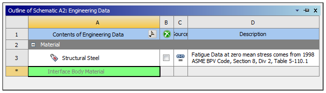
In the Static Structural schematic, right-click the Engineering Data cell and choose . The Engineering Data tab opens and displays Structural Steel as the default material.
Click the box labeled "Click here to add new material" and enter the name "Interface Body Material".
Expand the Linear Elastic option in the Toolbox and right-click Orthotropic Elasticity. Select . The required properties for the material are highlighted in yellow.
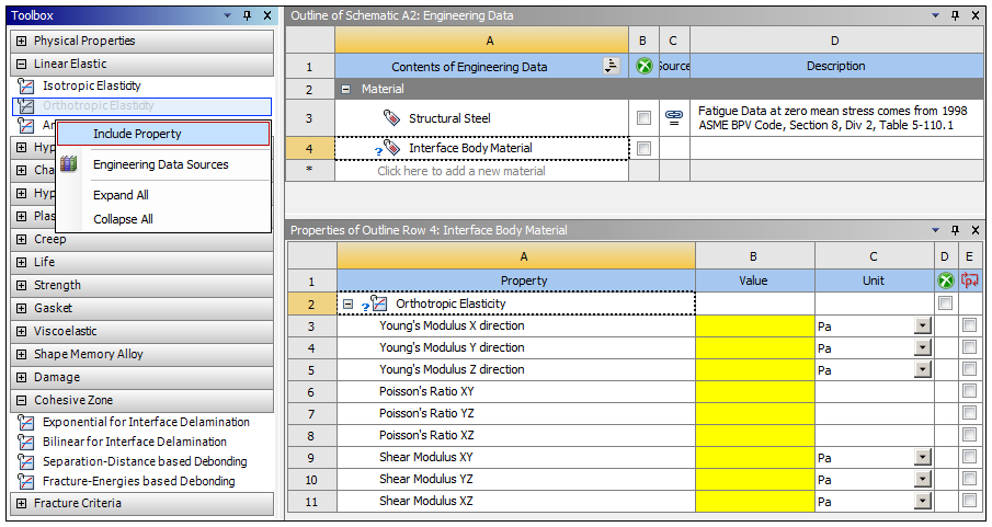
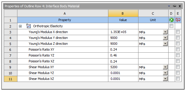
Define the new material by entering the following property values and units of measure into the corresponding fields.
Property Value Unit Young’s Modulus X Direction 1.353E+05 MPa Young’s Modulus Y Direction 9000 MPa Young’s Modulus Z Direction 9000 MPa Poisson’s Ratio XY 0.24 na Poisson’s Ratio YZ 0.46 na Poisson’s Ratio XZ 0.24 na Shear Modulus XY 5200 MPa Shear Modulus YZ 0.0001 MPa Shear Modulus XZ 0.0001 MPa The properties for the material should appear as follows:
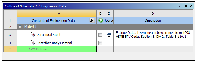
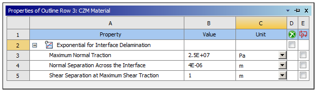
Click the box labeled "Click here to add new material" and enter the name “CZM Material”. This material will specify the formulation used to introduce the fracture mechanism (Cohesive Zone Material method).
Expand the Cohesive Zone option in the Toolbox and right-click . Select . The required properties for the material are highlighted in yellow.
Define the new material by entering the following property values and units of measure into the corresponding fields.
Property Value Unit Maximum Normal Traction 2.5E+07 Pa Normal Separation Across the Interface 4E-06 m Shear Separation at Maximum Shear Traction 1 m The properties for the material should appear as follows.
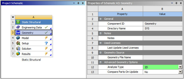
In the Static Structural schematic, right-click the Geometry cell and select >.
Browse to the proper location and open the file 2D_Fracture_Geom.agdb. This file is available here on the Ansys customer site.
Right-click the Geometry cell and select Properties. In the Properties window, set the Analysis Type property to .
The Project Schematic should appear as follows:
Launch Mechanical. Right-click the Model cell and then choose . (Tip: You can also double-click the cell to launch Mechanical).
Define unit system. From the Tools group on the Home tab, open the Units drop-down menu and select .
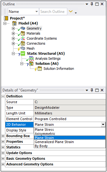
Define 2D behavior.
Highlight the Geometry object.
In the Details pane, specify the 2D Behavior property as . This constrains all of the UZ degrees of freedom. See the 2D Analyses section of the Mechanical User's Guide for additional information about this property.
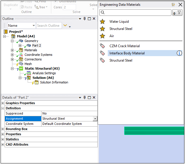
Apply Material: Expand the Geometry folder and select the Part 2 folder. Set the Assignment property to "Interface Body Material". Selecting the Part 2 folder allows you to assign the material to both parts at the same time.
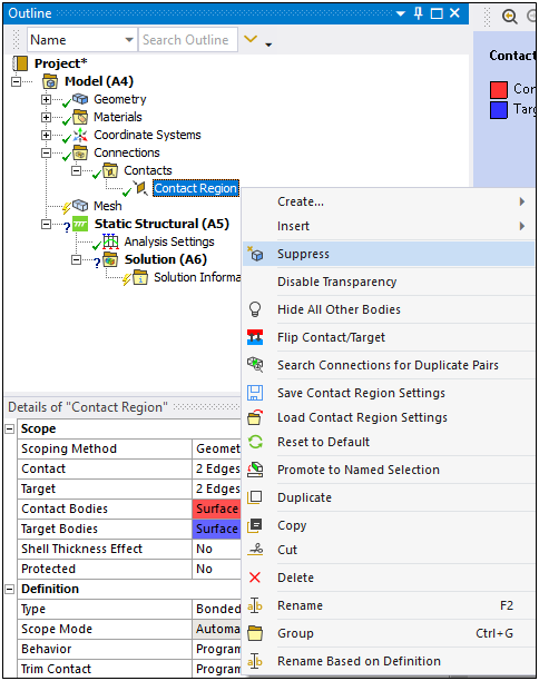
Suppress Contact.
Caution: Contact cannot be present for this analysis.
Expand the Connections folder and then expand the Contacts folder.
Right-click the Contact Region object and select .
This analysis requires a mesh property to match the elements of the two parts. To properly define the property, you need to define coordinate systems for the element faces that will be matched with one another. In theory, for this model, one coordinate system could facilitate the specification of the Mesh because the coordinate systems you are about to create are virtually identical.
Right-click the Coordinate Systems object in the tree and select >.
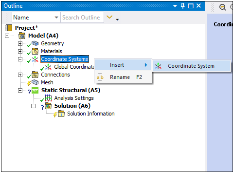
Right-click the new coordinate system object, select , and name the object "High Coordinate System."
In the Details pane of the newly-created Coordinate System object, select the Geometry property field Click to Change.
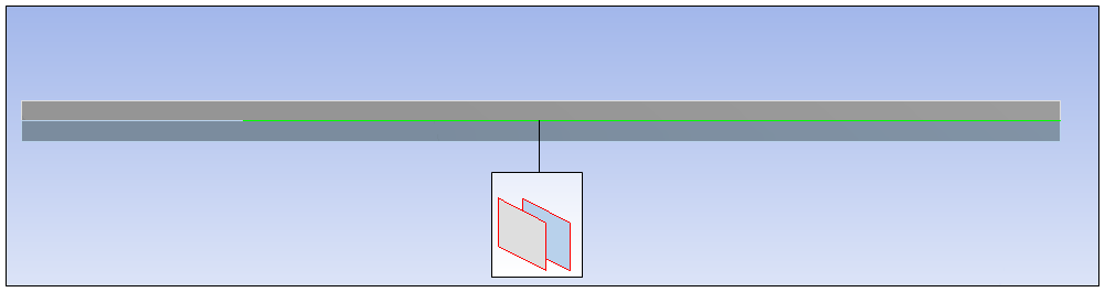
Select the Edge selection filter (on the Graphics Toolbar) and highlight an edge in the center of the model.
This tutorial employs the Depth Picking tool because of the close proximity of the two edges involved in the interface, as well as the crack. As illustrated here, the graphics window displays a stack of rectangles in the lower left corner. The rectangles are stacked in appearance, with the topmost rectangle representing the visible (selected) geometry and subsequent rectangles representing additional geometry selections. For this example, the topmost geometry is the "high" edge.
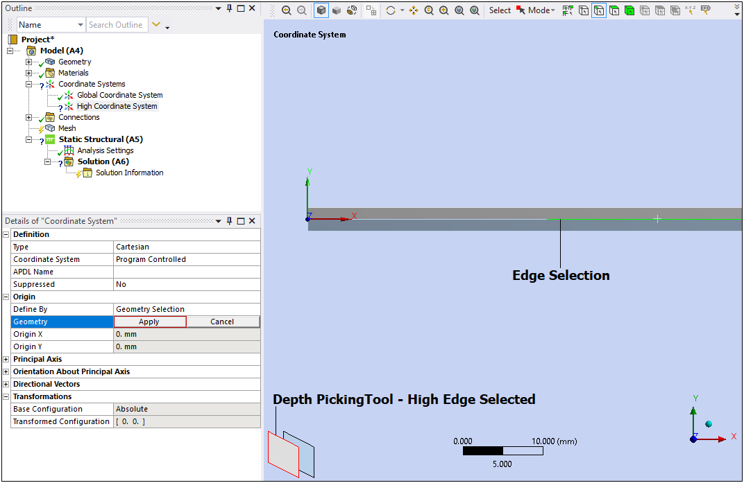
Click in the Geometry property. The "High Coordinate System" is defined.
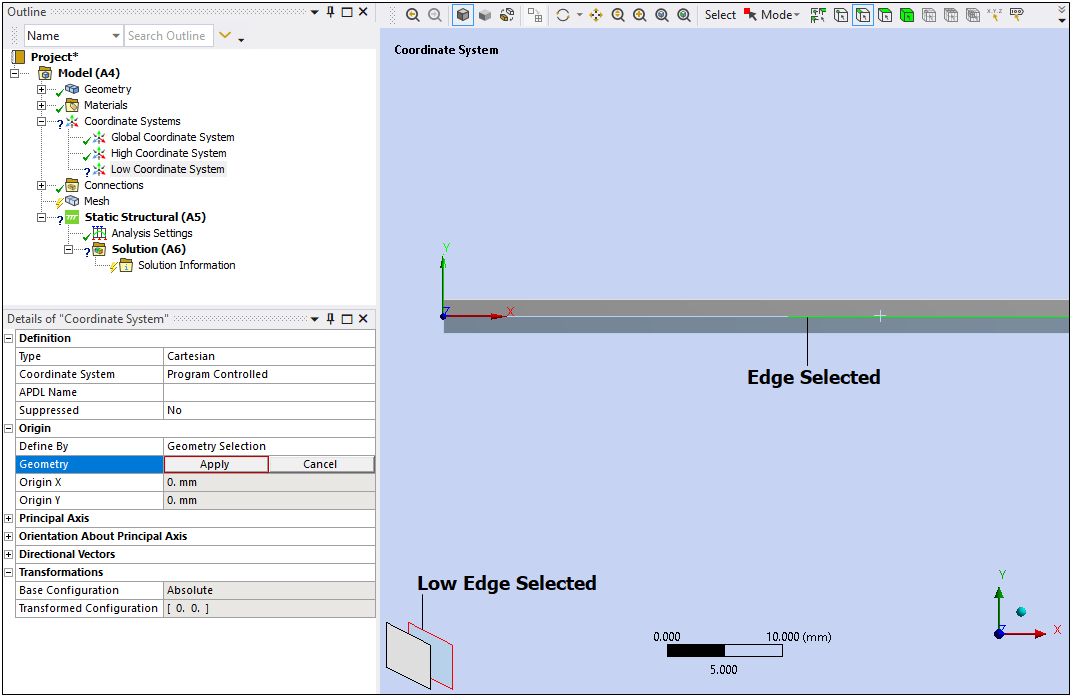
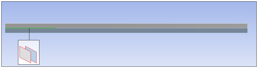
Right-click the Coordinate Systems object again and insert another object. Rename this object "Low Coordinate System."
Select the Edge selection filter and highlight an edge in the center of the model. Using the Depth Picking tool, select the second rectangle in the stack, and then scope the edge as the geometry ( in the Geometry property). This scoping is illustrated below.
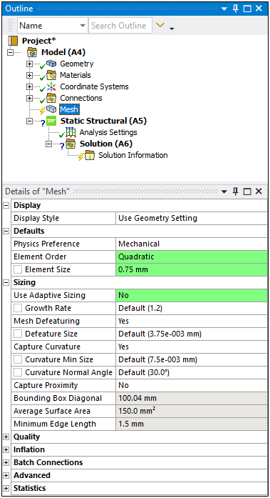
Select the Mesh object. Define the following Mesh object properties:
Set Element Order (Defaults category) to (kept).
Enter an Element Size (Defaults category) of
0.75.Set Use Adaptive Sizing (Sizing category) to
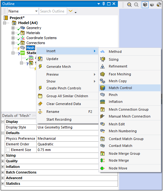
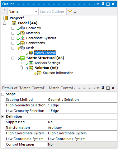
Right-click the Mesh object and select >.
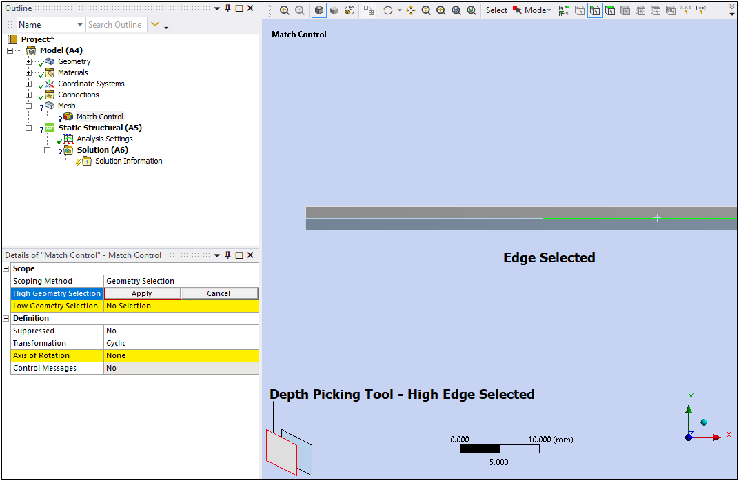
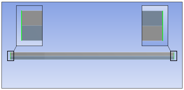
Activate the High Geometry Selection property by selecting its field (that is highlighted in yellow). The and buttons display. Select the Edge selection tool and highlight one of the edges in the center of the model. Use the Depth Picking tool to select the topmost geometry. Click the button.
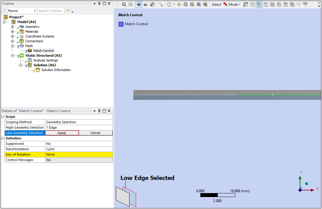
Perform the same steps to specify the Low Geometry Selection property, as illustrated below.
Change the Transformation property from to and specify the High Coordinate System and Low Coordinate System properties using the coordinate systems created in the previous step of the tutorial. The object should appear as illustrated below.
Select the Edge selection filter (on the Graphics Toolbar) and, holding the Ctrl key, select the four side edges.
Right-click the Mesh object and select >. This mesh sizing control should be scoped to the four side edges.
In the Details view, enter
0.75mm as the Element Size.Select the Edge selection filter (on the Graphics Toolbar) and highlight an edge in the center of the model. Use the Depth Picking tool and, holding the Ctrl key, select both rectangles in the lower left corner of the graphics window. Continue to hold the Ctrl key, and select an edge of the crack. Again, use the Depth Picking tool and select both rectangles in the lower left corner of the graphics window. Still holding the Ctrl key, select the top and bottom edges on the model.
Right-click the Mesh object and select >. This mesh sizing control should be scoped to six (top and bottom and the four interface edges) edges.
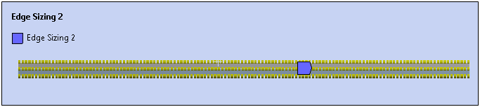
In the Details view, enter
0.5mm as the Element Size.Right-click the Mesh object and select .
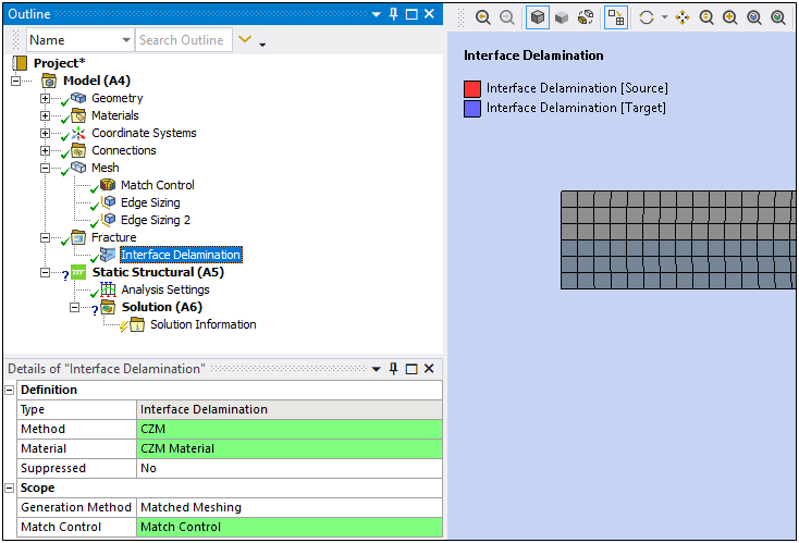
Insert a Fracture folder into the tree by highlighting the Model object and selecting the Fracture option from the Define group on the Model Context tab.
Select the option from the Model group on the Fracture Context tab.
In the Details pane, set the Method property to .
Set the Material property to .
Select the that was created earlier in the tutorial for the Match Control property.
The Interface Delamination object is complete.
Select the Analysis Settings object.
Set the Auto Time Setting property to and then enter
40for the Initial Substeps, Minimum Substeps, and Maximum Substeps properties.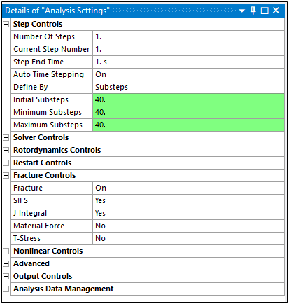
In the Details pane, set the Large Deflection property to to activate geometric nonlinearities.
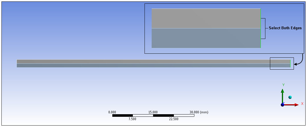
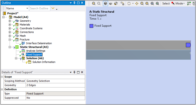
Select the Edge selection filter and select the two edges on the side of the model that is opposite of the crack. Select one edge, press the Ctrl key, and then select the next edge.
Highlight the Static Structural object and select the option from the Structural group on the Environment Context tab.
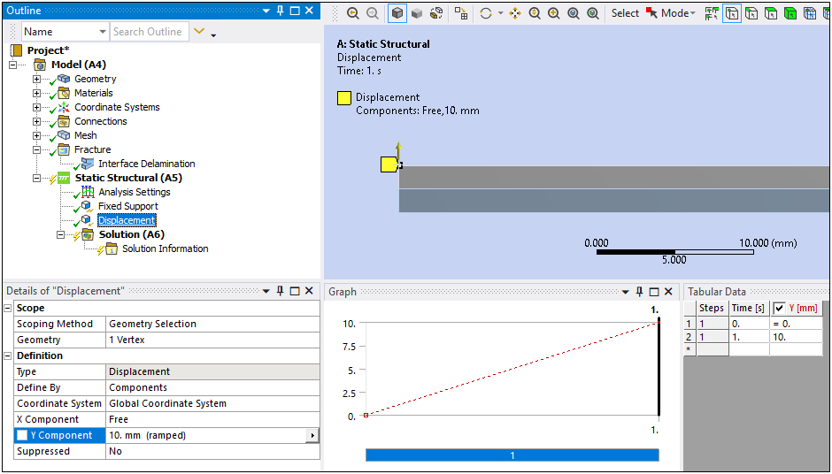
Highlight the Static Structural object. With the Vertex selection filter active, select the vertex illustrated below, and select the option from the Structural group on the Environment Context tab.
Highlight the object in the tree and enter 10 (mm in the positive Y direction) as the loading value for the Y Component property.
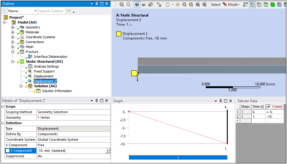
Create another . With the Vertex selection filter active, select the bottom vertex and select the option from the Structural group on the Environment Context tab. Enter -10 (mm in the negative Y direction) as the loading value for the Y Component property.
Highlight the Solution object. From the Results group of the Solution Context tab, open the Deformation drop-down menu and select Directional.
Under the Definition category in the Details view, set the Orientation property to .
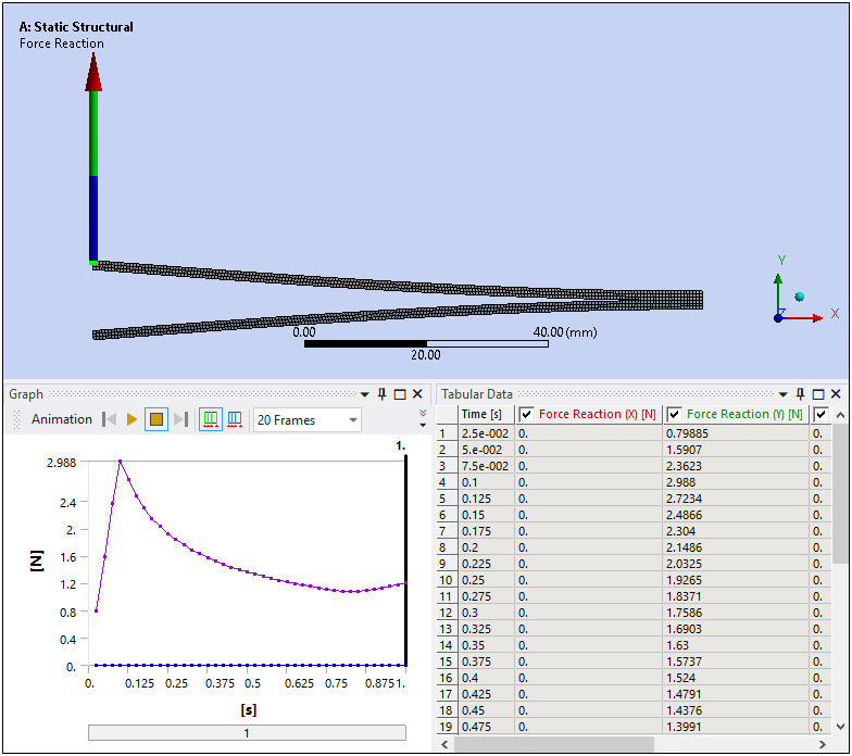
From the Results group of the Solution Context tab, open the Probe drop-down menu and select Force Reaction.
Select for the Boundary Condition property.
Click the button.
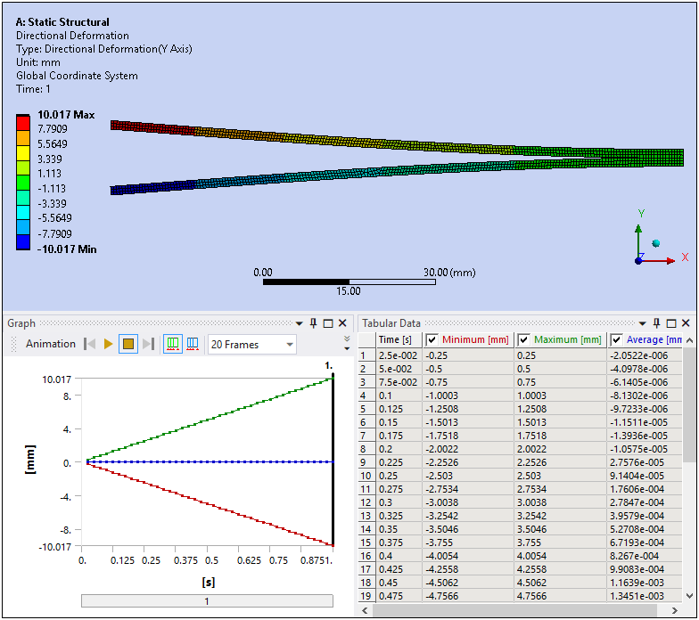
Highlight the Directional Deformation and Force Reaction objects. Results appear as follows:
You may wish to validate results against those outlined in the verification test case (VM248 in the Ansys Mechanical APDL Verification Manual). This is most easily accomplished by creating User Defined Results using the Worksheet.
Congratulations! You have completed the tutorial.