


This tutorial demonstrates the use of a nonlinear bushing to modify the behavior of a simple pendulum.
| Analysis Type | Rigid Dynamics |
| Features Demonstrated | Nonlinear bushings, reference coordinate system, mobile coordinate system |
| Licenses Required | Ansys Mechanical Premium/Enterprise/Enterprise PrepPost |
| Help Resources | Bushing Joint |
| Tutorial Files | simple_pendulum.zip |
This tutorial guides you through the following topics:
Prepare the analysis system.
Browse to open the file NLBushingTuto.wbpz. A Rigid Dynamics system will populate the Project Schematic. This file is available here on the Ansys customer site.
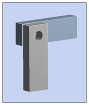
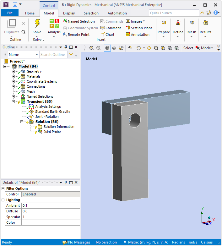
Right-click the Model cell, and select to open the Mechanical Application. The model shown below will open.
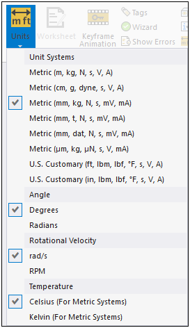
Set the units system.
From the Tools group of the Home tab, open the Units drop-down menu and specify the following:
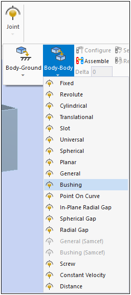
Insert a new bushing.
Open the Connections folder and select the Joints object.
From the Joint group of the Connections Context tab, open the Body-Body drop-down menu, and select .
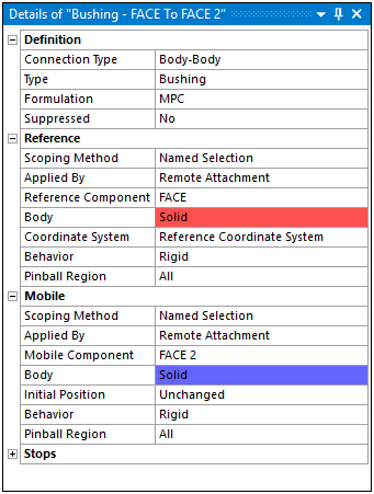
Scope the bushing to the correct faces:
Set the Scoping Method property of the Reference category to .
Set the Reference Component property to .
Set the Scoping Method property of the Mobile category to .
Set the Mobile Component property to .
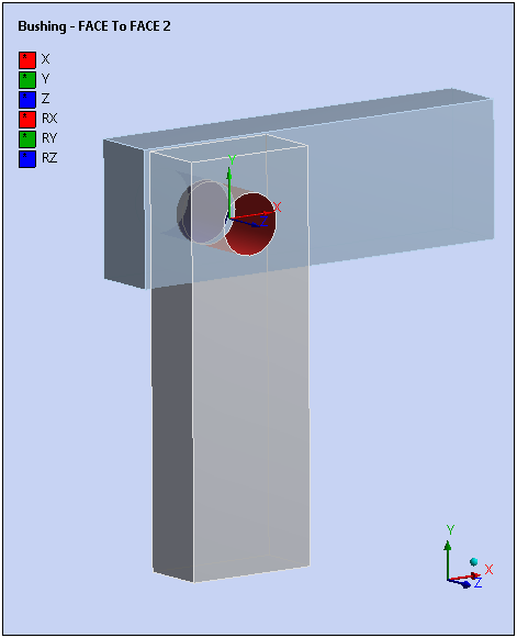
The bushing Reference Coordinate System should now be defined as illustrated here. Note that the pendulum axis of rotation is the Z-axis.
Add a nonlinear rotational stiffness to the Z axis
In the Outline, highlight the new bushing, then toggle the Worksheet view.
In the Bushing worksheet, right-click the last diagonal term of the Stiffness Matrix, and select Tabular.
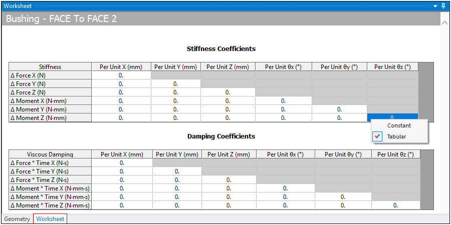
Note that only the diagonal terms of the stiffness matrix can be defined as nonlinear.
In the Tabular Data window, enter the angle and moment data pictured below:
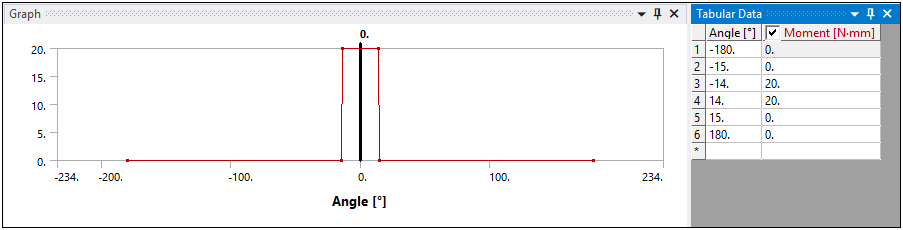
The curve defined is also displayed in the Graph window.
Solve the model.
Select the option.
Observe the defined nonlinear behavior.
In the Outline, select the Joint Probe object under the Solution object to view the pendulum motion animation. Select the option in the window to animate the result. The pendulum should oscillate near its initial horizontal position due to the high stiffness entered for small angular displacements.
With joint rotation unsuppressed, a 20° rotation of the pendulum will occur at the beginning of the analysis, and the pendulum should have free oscillation around the vertical axis.
Congratulations! You have completed the tutorial.