


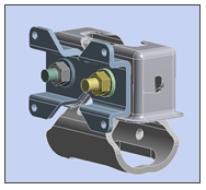
This tutorial demonstrates the use of Finite Element (FE) types exposed in the Mechanical application by resolving an overconstraint issue in a static structural analysis of a bracket assembly with contacts.
| Analysis Type | Static Structural |
| Features Demonstrated | Node-based Named Selections, worksheet criterion, selection tool, FE (node-based) boundary conditions, FE connections, FE nodes, Solution Information worksheet |
| Licenses Required | Ansys Mechanical Pro/Premium/Enterprise/Enterprise PrepPost |
| Help Resources | Setting Connections |
| Tutorial Files | Bracket_Assembly.agdb |
This tutorial guides you through the following topics:
Create Static Structural Analysis.
Open Ansys Workbench.
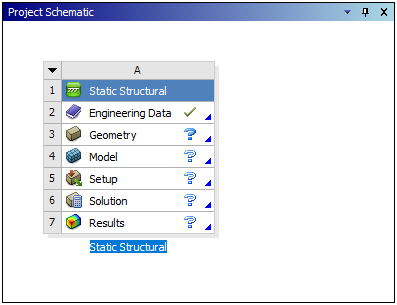
On the Workbench Project page, drag a Static Structural system from the Toolbox to the Project Schematic. The Project Schematic should appear as follows:
Assign Materials.
For this tutorial we will accept Structural Steel (typically the default material) for the model and add Aluminum Alloy as a material option.
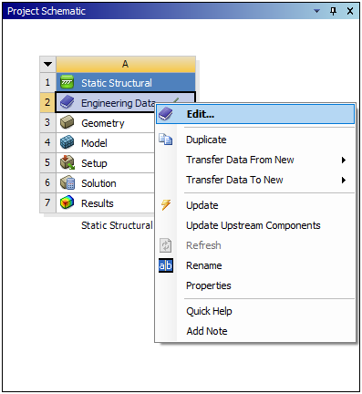
In the Static Structural schematic, right-click the Engineering Data cell and select Edit. The Engineering Data tab opens and displays Structural Steel as the default material.
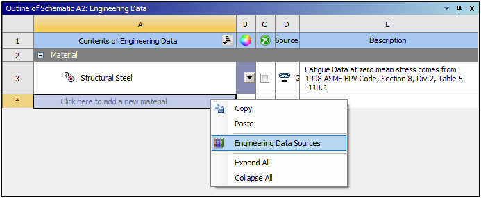
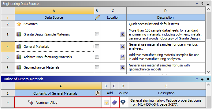
Right-click the box below Structural Steel, where it says "Click here to add new material" and select Engineering Data Sources.
Select General Materials and click the Add button for Aluminum Alloy. A book icon appears in the column next to the Add button (plus symbol) to indicate that the material is selected.
Return the Project Schematic.
Attach Geometry.
In the Project Schematic, right-click the Geometry cell and select > .
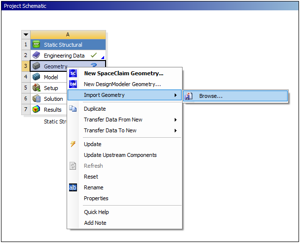
Browse to the proper location and open the file Bracket_Assembly.agdb. This file is available here on the Ansys customer site.
Launch Mechanical by right-clicking the Model cell and then selecting Edit. (Tip: You can also double-click the cell to launch Mechanical).
Define Unit System: from the Tools group on the Home tab, open the Units drop-down menu and select .
Define Part Material and Create Named Selection.
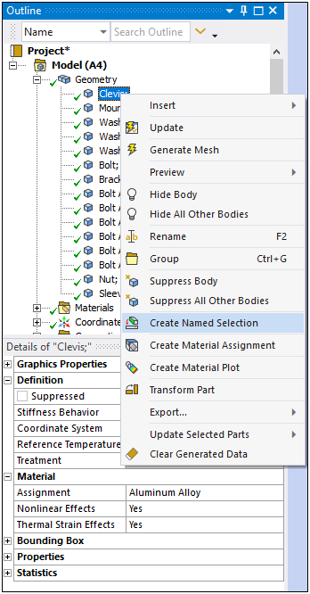
For this model, all of the parts have been defined as Structural Steel. However, we want to change the Material type of the Clevis to Aluminum Alloy. To do this, first expand the Geometry object in the tree.
Select the Clevis object under Geometry. In the Details under the Material category, select the fly-out menu of the Assignment property and select Aluminum Alloy.
Right-click Clevis object and select . Enter the Selection Name"Clevis" and click the button.
Define Connections.
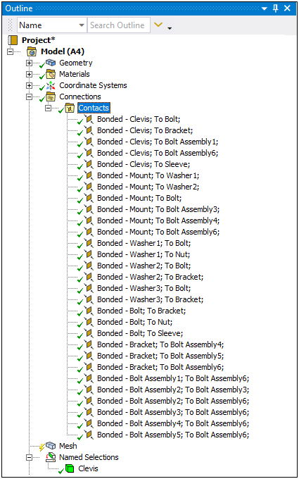
Expand the Connections folder and then expand the Contacts folder.
Right-click the Contacts folder and select .
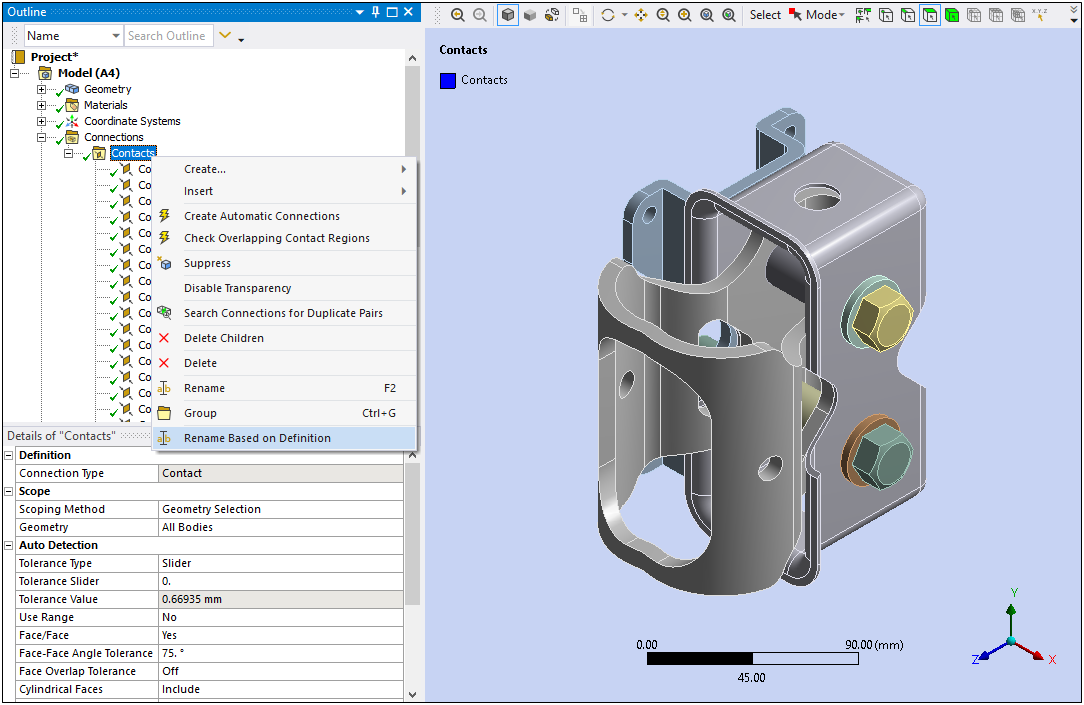
The renamed contact conditions are illustrated below.
To create and modify node-based boundary conditions, you must first generate the model’s mesh. In addition, for this example, we will use the Body Sizing feature to define certain local mesh sizing.
Insert Body Sizing.
Select the Mesh object and specify the Element Size as 2 (mm).
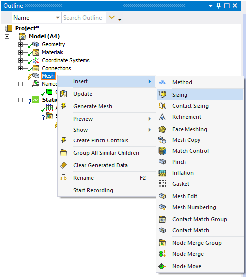
Right-click the Mesh object and select > .
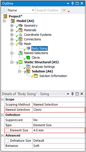
In the Details view, set the Scoping Method property to .
Select the Named Selection field and select from the drop-down menu.
In the Element Size field, enter 4 (mm).
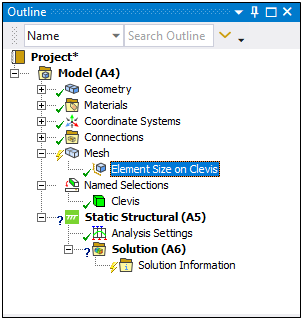
Right-click the object and select .
As illustrated here, the object is renamed.
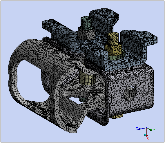
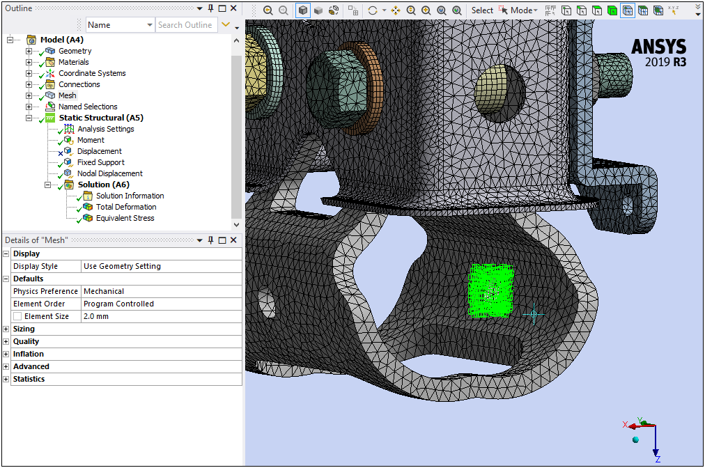
Generate Mesh: Right-click the Mesh object select .
The completed mesh is shown here.
Specify the following boundary conditions:
Moment
Displacement
Fixed Support
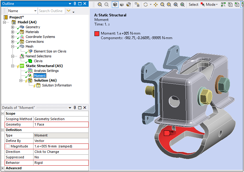
Insert a Moment Load.
Select the Static Structural object, right-click, and select >.

Select the inner face of the Clevis (1 Face) as illustrated here. In the Details for the Scope category, select the Geometry field and click . Enter 1e5 N mm as the Magnitude and change the Behavior to Rigid.
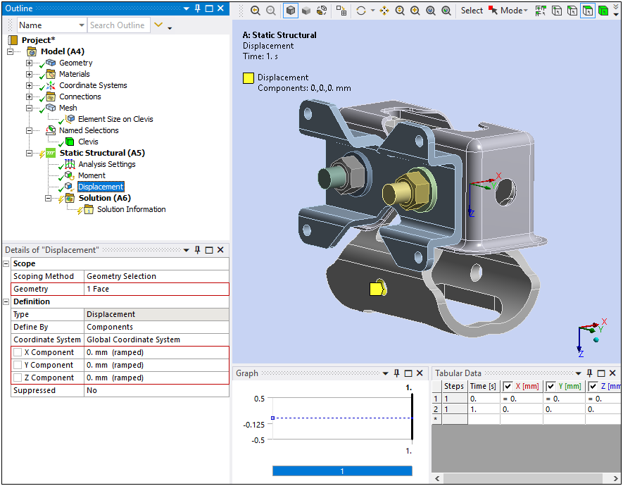
Insert a Displacement and Fixed Support.
With the Moment object still highlighted, right-click, and select >.
Select the inner face of the circular hole highlighted here. Make sure that the model is oriented as shown (note the direction of the bolts) and then click the button in the Geometry field. Set the values of X Component, Y Component, and Z Component, to 0 mm.
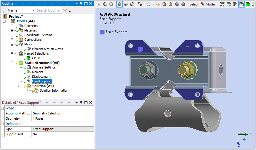
Finally, let’s immobilize the assembly by specifying Fixed Supports on the faces illustrated below. From the Structural group of the Environment Context tab, select , select one of the faces, press and hold the Ctrl key, and then select the remaining three faces. Once all of the faces are selected, click the button in the Geometry field.
This section outlines the steps to add result objects, solve your analysis, and review your results.
Specify Result Object and Solve.
Highlight the Solution object, right-click, and select the > Deformation > .
Right-click the Solution object and select .
Review the Results.
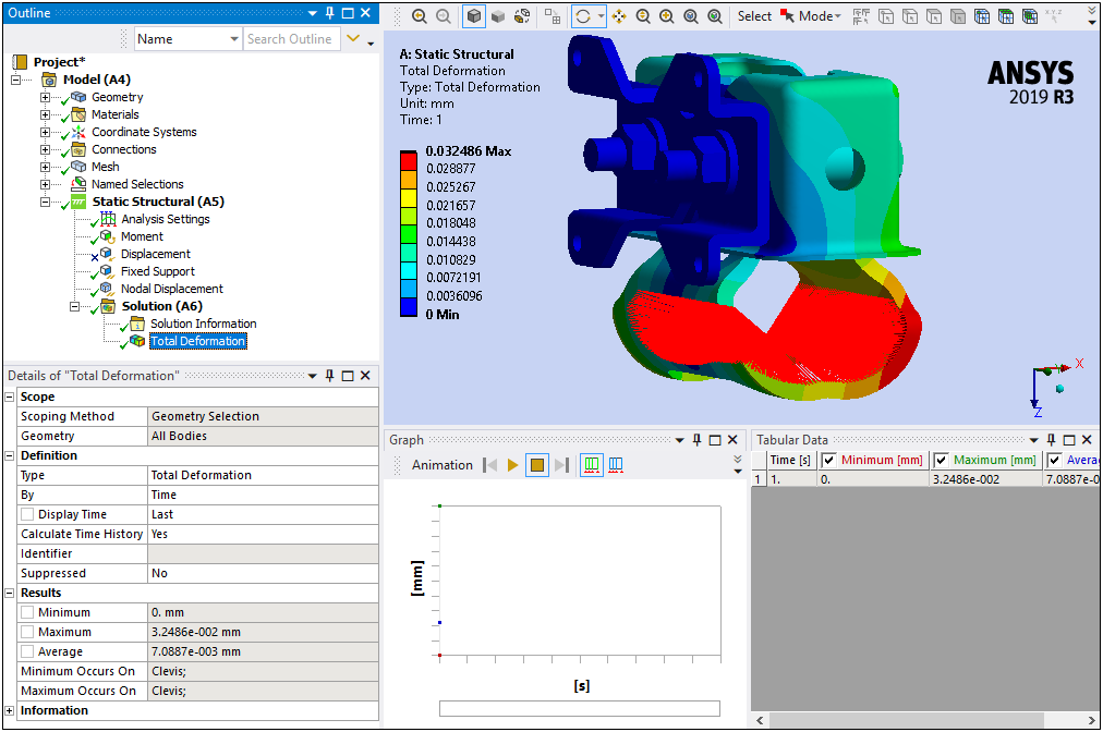
Select the Total Deformation object. The solved model should display as follows:
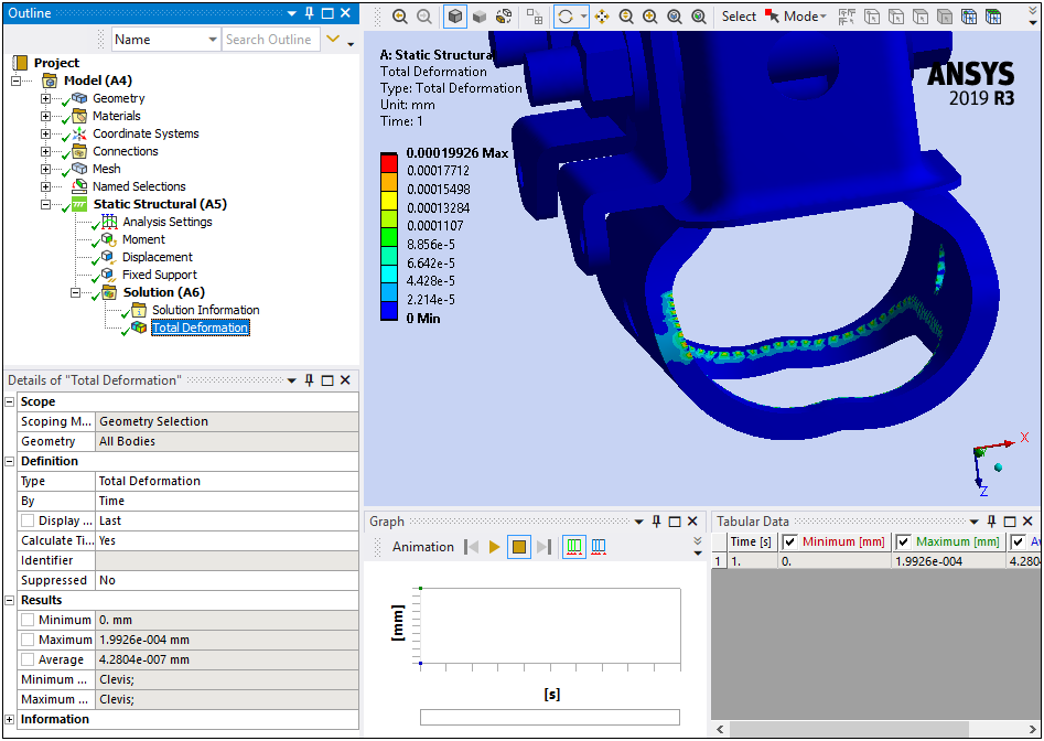
The bulk of the result displays in blue, indicating no deformations on the assembly. This cannot be correct. In addition to that condition, the following Warning Message displays:
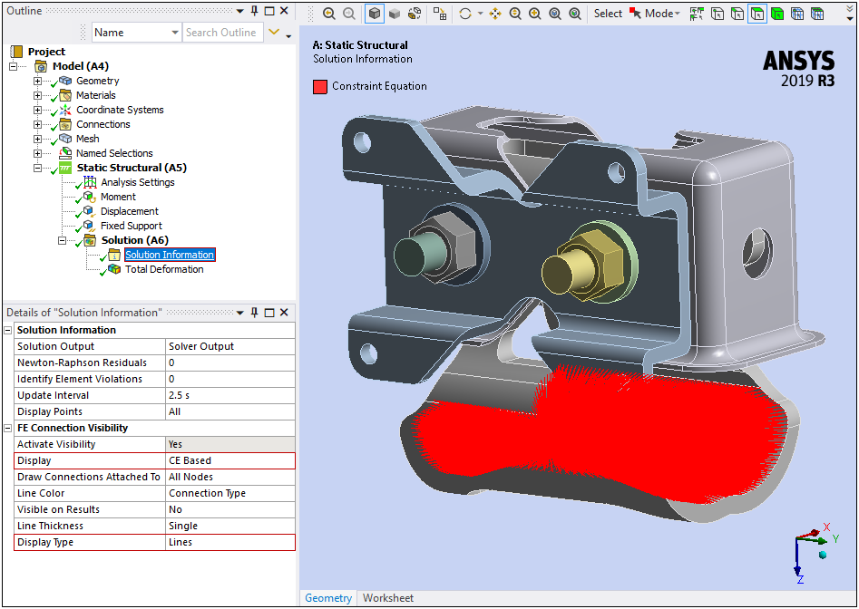
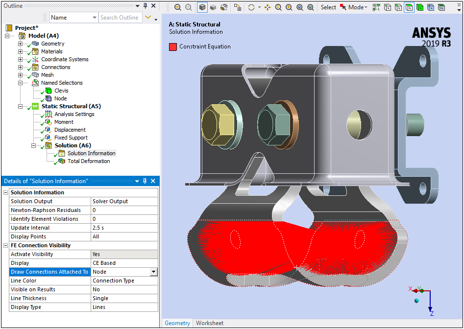
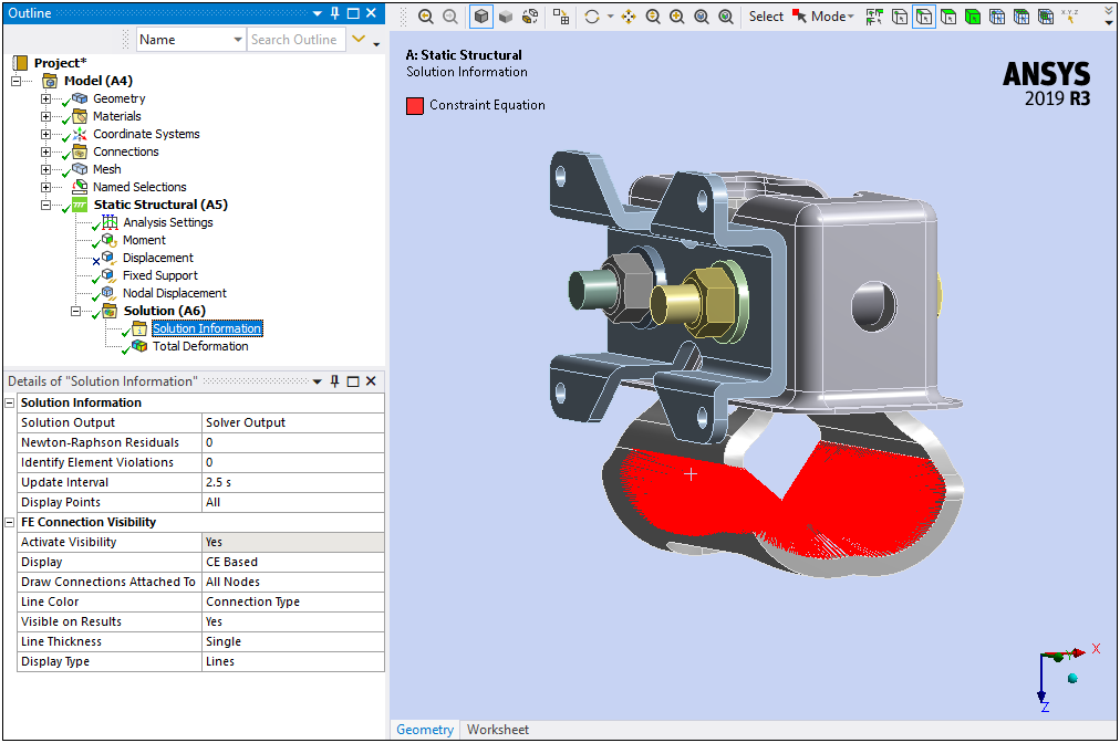
One or more MPC contact regions or remote boundary conditions may have conflicts with other applied boundary conditions or other contact or symmetry regions. This may reduce solution accuracy. Tip: You may graphically display FE Connections from the Solution Information Object for non-cyclic analysis. Refer to Troubleshooting in the Help System for more details. You can graphically display FE Connections from the Solution Information object (Geometry tab), as illustrated below. In the Details, specify the Display property as and the Display Type as . As you can see there is an abundance of Constraint Equations.
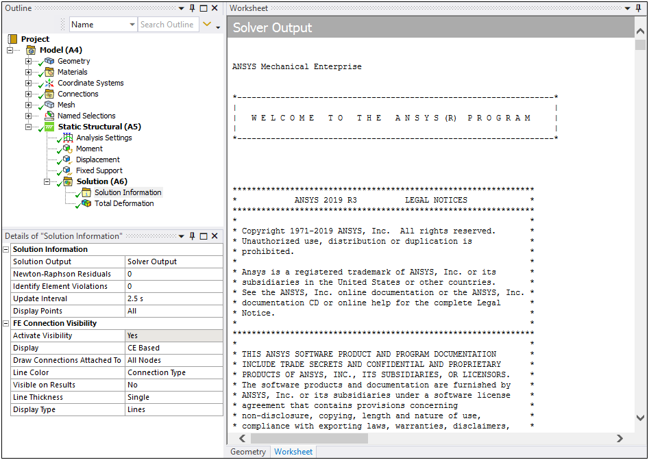
Now, let’s look at Solver Output to track down the overconstraint issue.
Display the Worksheet of the Solution Information object. The contents of the Worksheet display output messages, including Warnings. Scroll through the messages, searching for overconstraint messages/warnings.
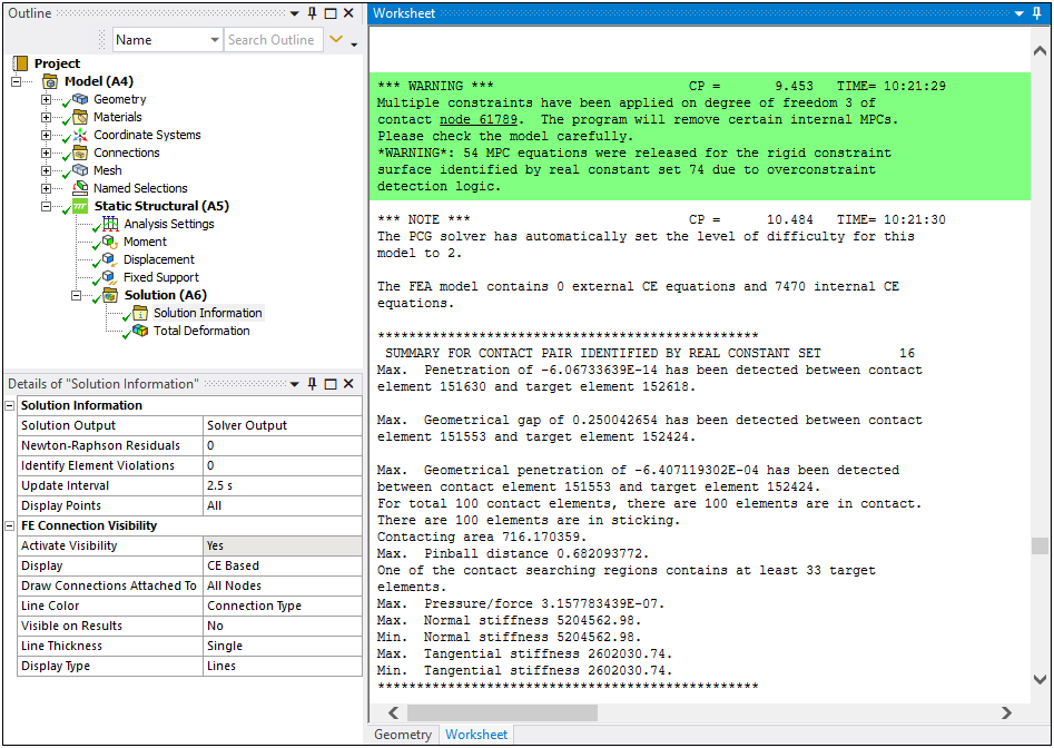
The warning highlighted here provides a starting point to correct the overconstraint. A node is identified as a node that is overconstrained; specifically that it has multiple constraints on degree of freedom 3. In this example, the identified node is node 61789. Based on the version of the software you are using, this node value could change. For the purposes of this tutorial, we will use node 61789.
FE access makes it possible to select a single node using the Node ID. That is, the Mechanical application allows us to create a Named Selection for the identified node so we can that identify it specifically and view it graphically.
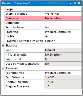
Select the Named Selections object and then select the Named Selection option from the Insert group of the Named Selections Context tab. A Selection object is generated. In the Details for the Selection object, change the Scoping Method to . The Worksheet view automatically displays.
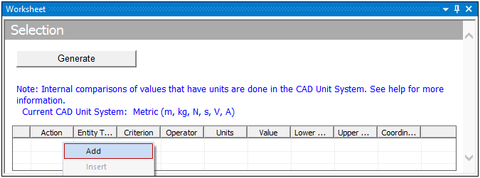
Right-click in the first row of the table and select .
Specify the criteria as follows:
Entity Type =
Criterion =
Operator =
Value =
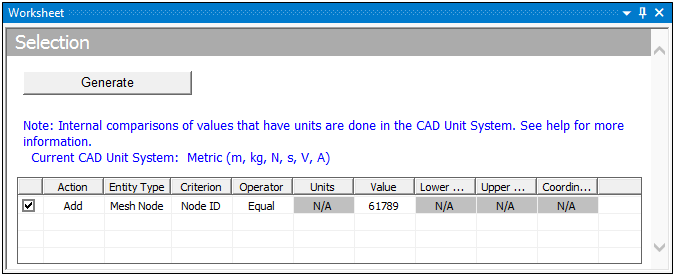
Click the button.
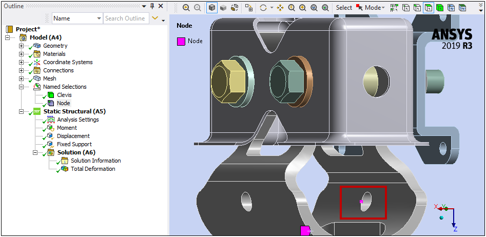
Right-click Selection and select . Change the name to "Node". A selection is generated that is just the one node that is overconstrained. Select the Graphics tab to view the generated node.
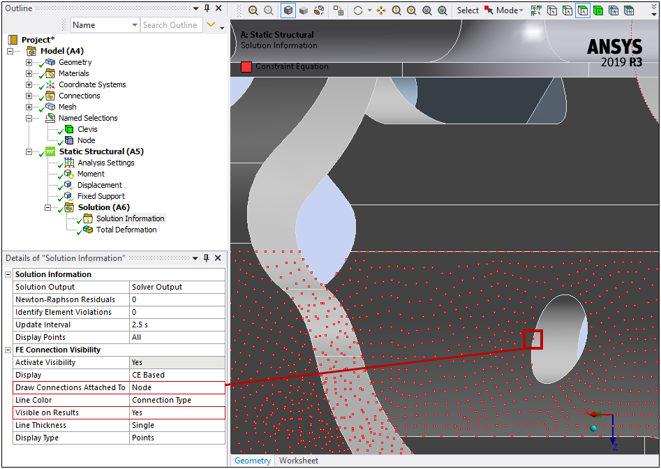
With node-based Named Selections, it is possible to view the Constraint Equations (CEs) attached to a single node. Select Solution Information object, select the Geometry tab at the bottom of the window, and then select as the option for the property, Draw Connections Attached To.
You should see the following illustration. The CEs are displayed as lines (note Display Type in the Details).
Set the Display Type property to , as illustrated below. You can see the specified Node as well as all of the other nodes used to calculate CEs. All nodes other than the specified node hollow. This indicates that each node is connected to the specified node.
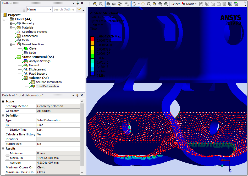
In addition, the Visible on Results property has been set to . This facilitates the display of the contour results for the Total Deformation result and the CEs, also shown below.
Here is an illustration of the CEs while the Total Deformation object is selected.
We have identified the overconstrained node, now, let’s correct the issue.
A starting point to correct the overconstraint is to remove the Displacement at Node 390. But looking at the scoping of the Moment and Displacement, it is clear that they share the edge nodes on the hole on the side of the face where the Moment is applied. As a result, when the CE's are generated from the Moment load, the solver tries to impose displacements on the edge nodes which may conflict with the Displacement already imposed due to the Displacement constraint. So, it is reasonable to try to remove the Displacement on the edge nodes. While a typical Displacement Boundary Condition does not allow for this option, it can be accomplished with Nodal Displacement.
Create Geometry-based Named Selection.
Select the Named Selections object and then select the Named Selection option from the Insert group of the Named Selections Context tab. A Selection object is generated.
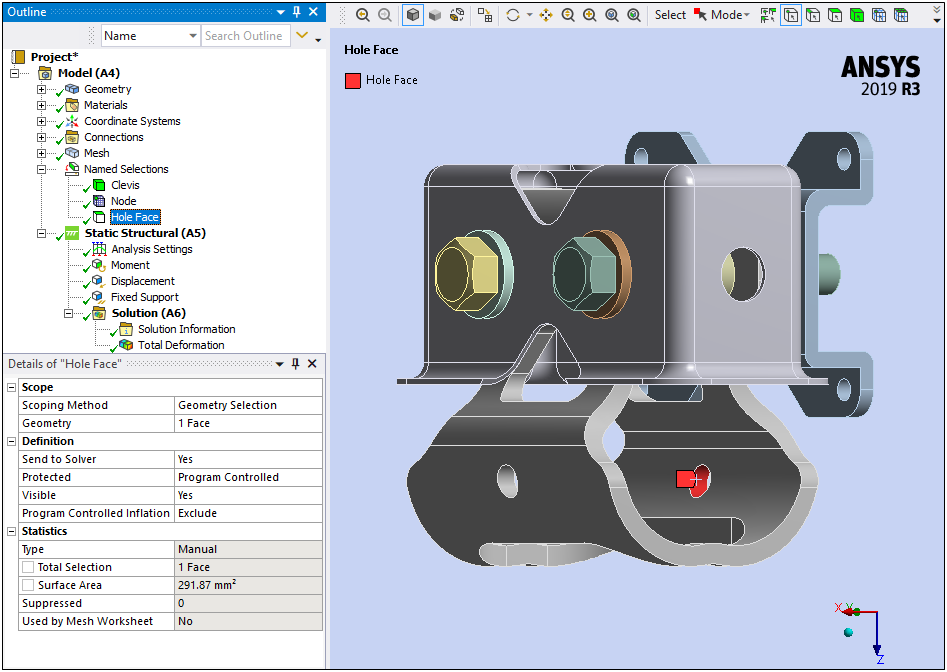
Make sure that the Face selection toolbar option is chosen and then select the hole in the Clevis. In the Details for the Selection object, the Scoping Method should be set to . In the Geometry field, click the button to specify the hole as the Geometry.
Right-click Selection and select . Change the name to "Hole Face".
Create Node-based Named Selection.
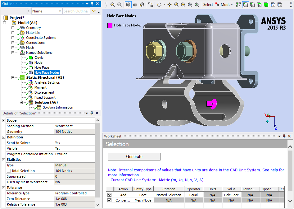
Right-click the "Hole Face" Named Selection and select the option. A new Selection object is generated.
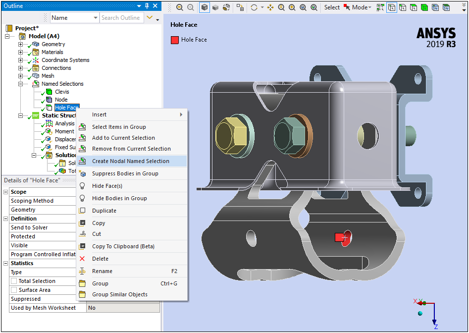
Right-click the new Selection object and select . Change the name to "Hole Face Nodes".
Convert Edge to Nodes and Remove it from the Geometry. Now, let’s use a criterion-based Named Selection to create a Named Selection for the hole that subtracts (removes) the nodes of the hole’s edge.
Insert a new Named Selections object.
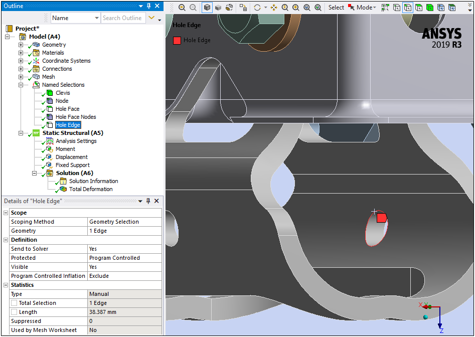
Using the Edge selection filter, select the edge of the hole. In the Details for the Selection object, the Scoping Method should be set to . Specify the edge using the Geometry property.
Right-click Selection and select . Change the name to "Hole Edge".
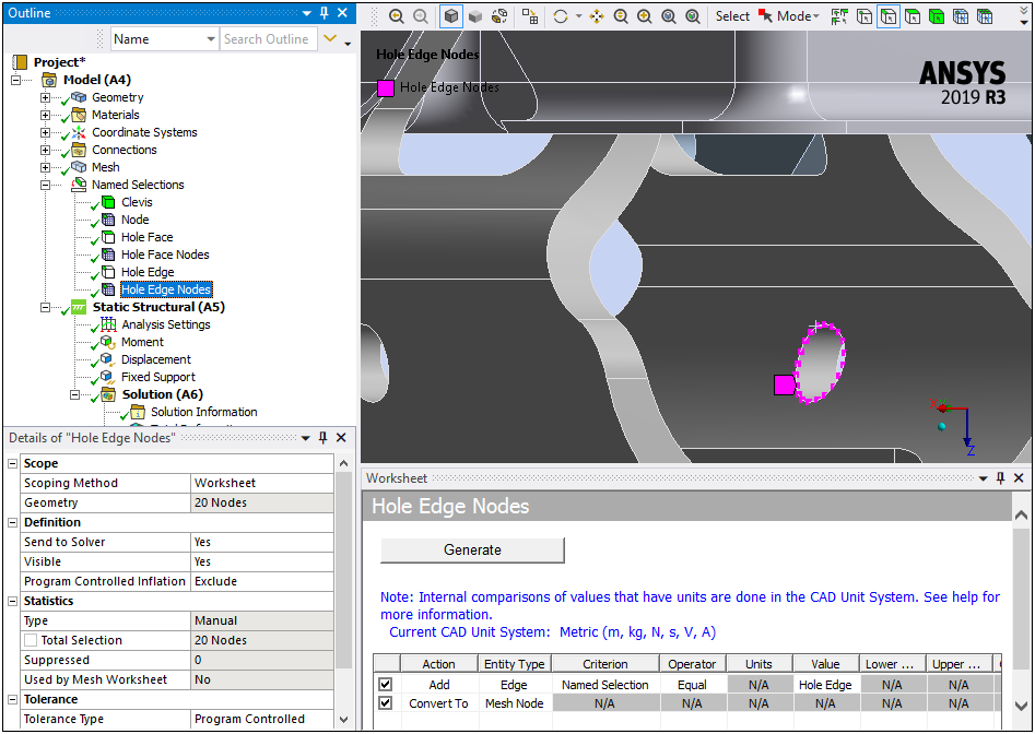
Right-click the "Hole Edge" Named Selection and select the option. A new Selection object is generated.
Right-click the new Selection object and select . Change the name to "Hole Edge Nodes".
One more Named Selection is required. This Named Selection will remove the edge nodes from the hole nodes.
Insert a new Named Selection object. A new Selection object is generated.
Right-click the new Selection object and select . Change the name to "Hole Face Minus Edge".
In the Details for the Selection object, change the Scoping Method to . Specify the criteria as illustrated here and then click the button.
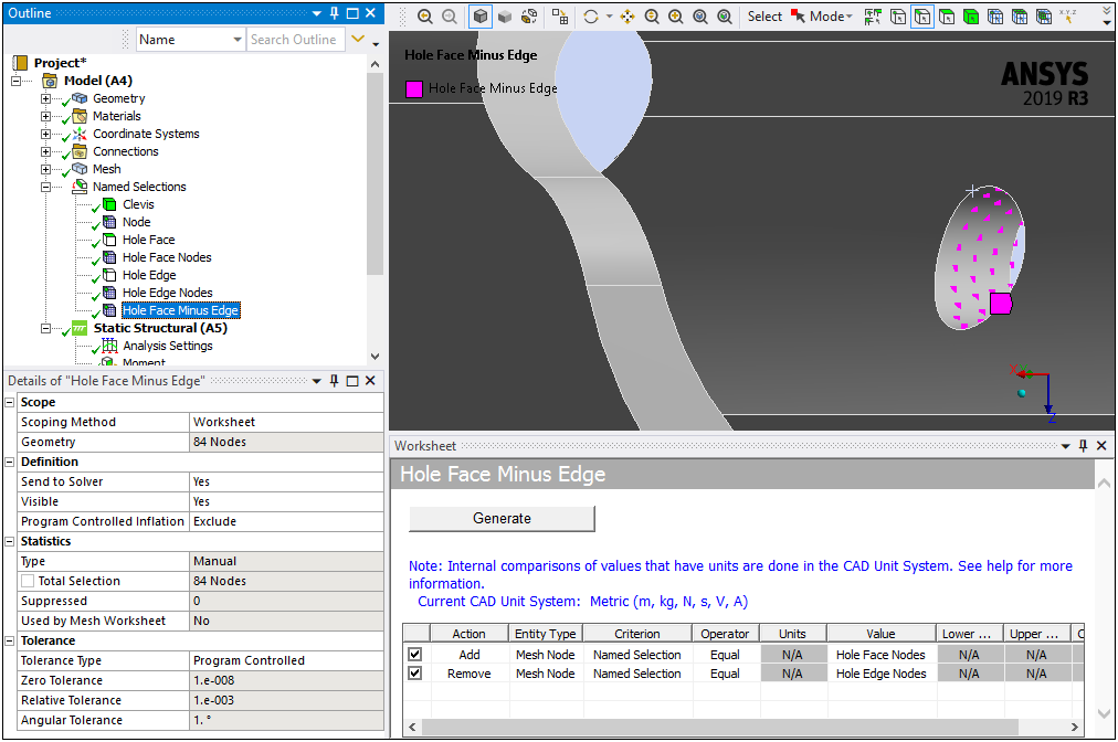
We now have a node-based Named Selection that includes all of the nodes of the hole, minus the nodes of the inner edge of the hole.
Suppress the existing Displacement: select the Displacement object, right-click, and select . If desired, you could instead delete the load.
Create Nodal Displacement and Solve. Now let’s define the scope of the Nodal Displacement and re-solve the analysis.
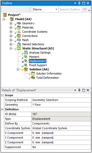
Right-click the Static Structural object and select > .
Node-based boundary conditions can only be scoped to Named Selections. In the Details for the , specify as the Named Selection and then specify each Component (X, Y, and Z) as 0.
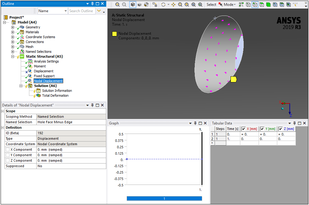
Click the button.
The solution should appear as shown here.
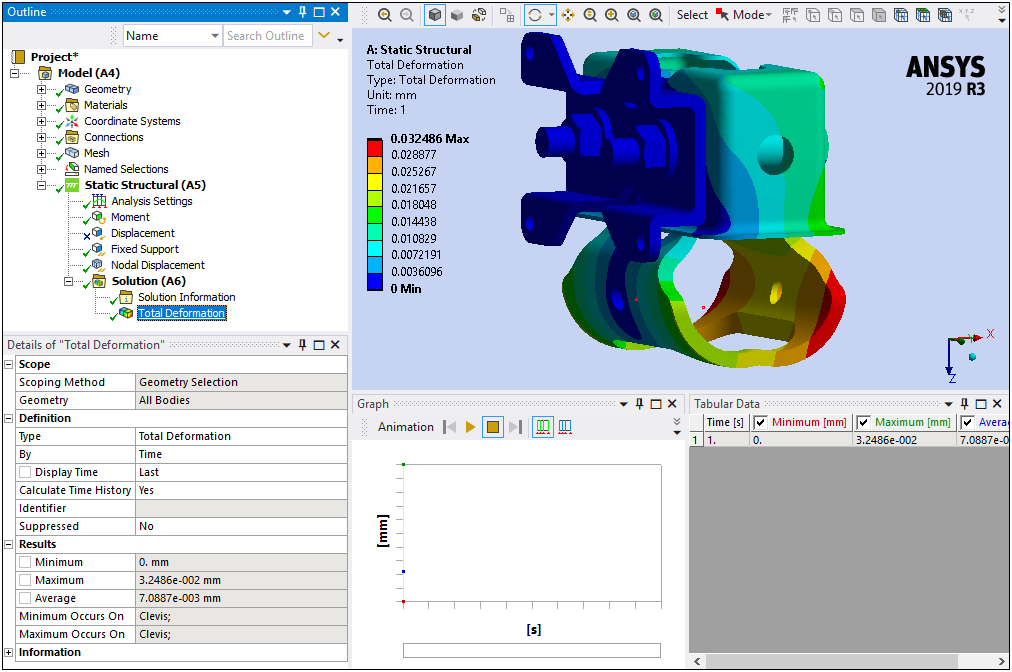
The Constraint Equations should appear with a uniform pattern, as illustrated here for the Solution Information object. And once again, the Visible on Results control has been set to so that you can view Constraint Equations and contour results (make sure to select the Geometry tab).
Examine Equivalent Stresses. Now, let’s examine the Equivalent Stresses on the model.
Right-click the Solution object and select > > .
Right-click the new result and select . The result should appear as illustrated here.
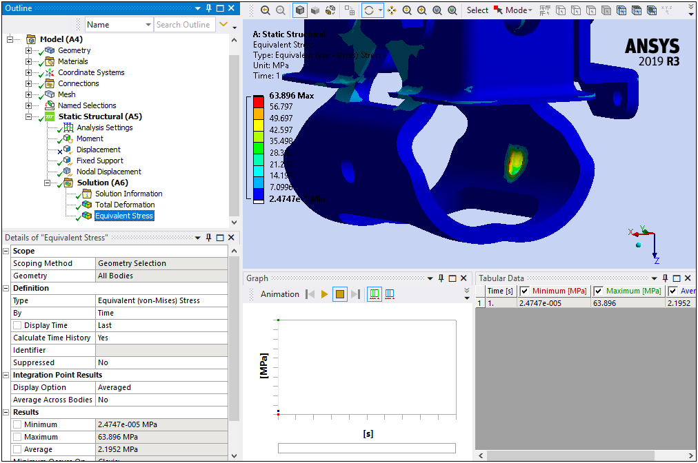
A zero Displacement was applied and this is reflected in the above result.
Examine the stresses on the hole using direct node selection.
Graphically Select Nodes.
Select the Mesh object and then select the Node selection filter from the Graphics Toolbar.
Open the Mode drop-down menu on the Graphics Toolbar and choose .
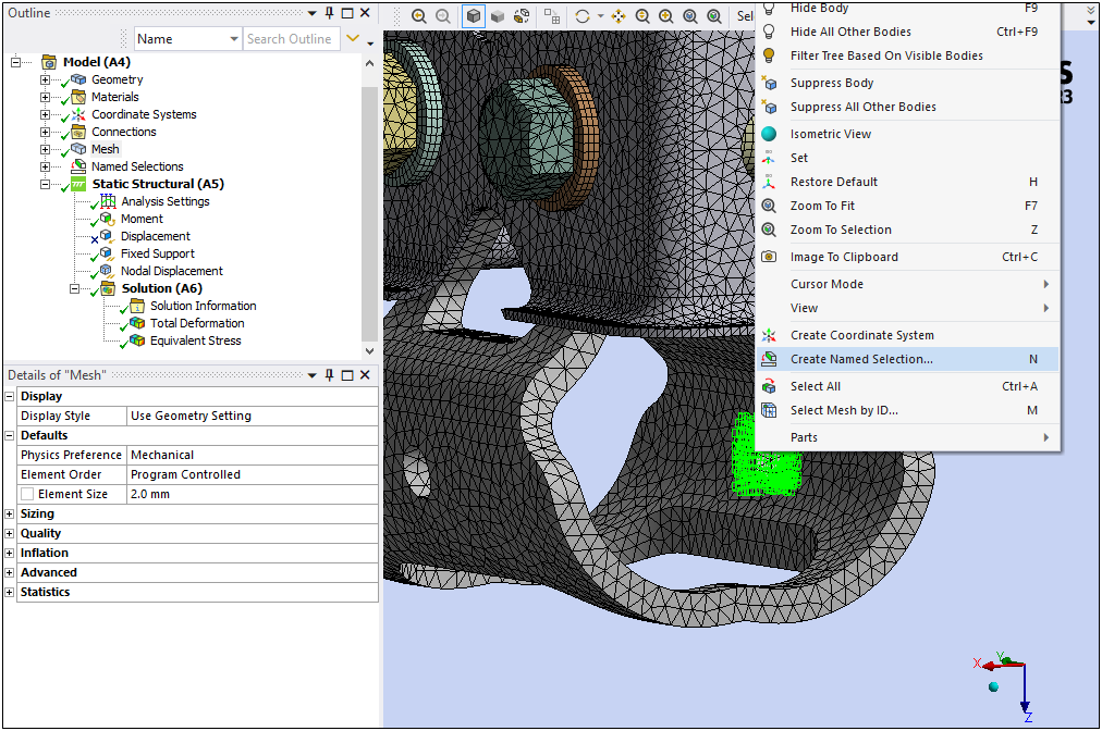
Drag your cursor over the Clevis hole in a pattern similar to what is illustrated here to directly select the nodes in and around the hole.
Right-click the mouse and select Named Selection. Enter "Stress Nodes" as the Selection Name.
Select the Equivalent Stress object, right-click, and select .
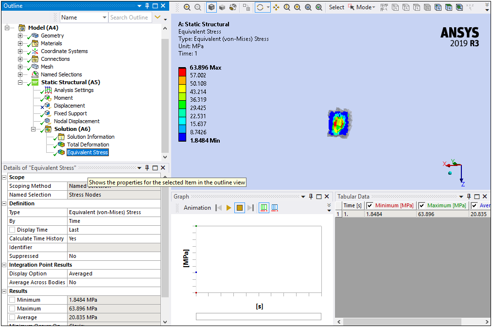
Scope the Equivalent Stress result to the Stress Nodes Named Selection (Scoping Method = and the Named Selection = ).
Right-click the Equivalent Stress object and select . The result should display as shown here.
Congratulations! You have completed the tutorial.