


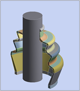
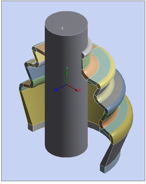
This example of a rubber boot seal demonstrates geometric nonlinearities (large strain and large deformation), nonlinear material behavior (rubber), and changing status nonlinearities (contact). The objective of this example is to show the advantages of the surface-projection-based contact method and to determine the displacement behavior of the rubber boot seal and stress results.
| Analysis Type | Nonlinear Static |
| Features Demonstrated | Hyperelastic material creation, remote point, Named Selections, manual contact generation, large deflection, multiple load steps, nodal contacts |
| Licenses Required | Ansys Mechanical Premium/Enterprise/Enterprise PrepPost |
| Help Resources | Chapter 26: Nonlinear Analysis of a Rubber Boot Seal |
| Tutorial Files | BootSeal_Cylinder.agdb |
This tutorial guides you through the following topics:
This is the same problem given in Chapter 26: Nonlinear Analysis of a Rubber Boot Seal in the Mechanical APDL Technology Showcase: Example Problems. It is provided here to illustrate the steps to set up and analyze the same model using the Mechanical application.
A rubber boot seal with half symmetry is considered for this analysis. There are three contact pairs defined; one is rigid-flexible contact between the rubber boot and cylindrical shaft, and the remaining two are self contact pairs on the inside and outside surfaces of the boot.
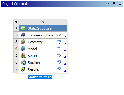
Create a Static Structural analysis system.
Start Ansys Workbench.
On the Workbench Project page, drag a Static Structural system from the Toolbox to the Project Schematic.
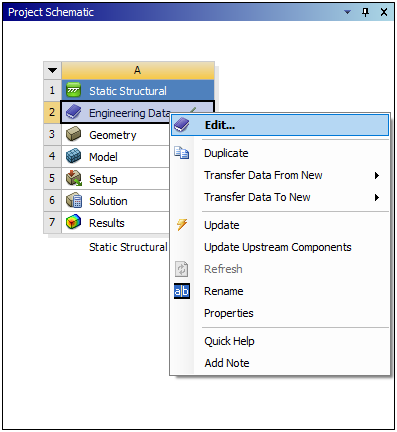
Create Materials.
Follow the given steps to create a material to use during the analysis.
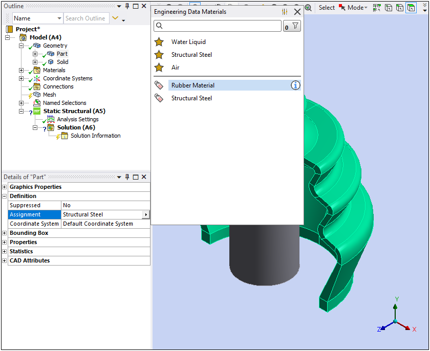
In the Static Structural schematic, right-click the Engineering Data cell and choose . The Engineering Data tab opens. Structural Steel is the default material.
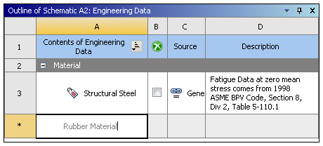
From the Engineering Data tab, place your cursor in the Click here to add new material field and then enter "Rubber Material".
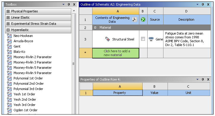
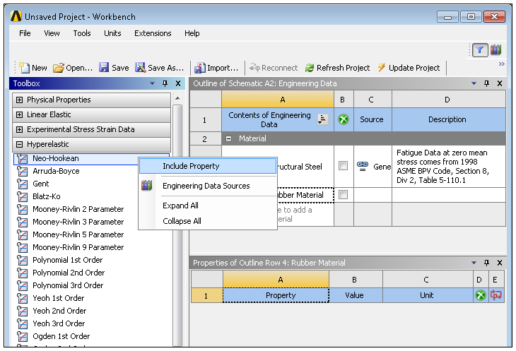
Expand the Hyperelastic Toolbox menu:
Select the option, right-click, and select .
Enter
1.5for the Initial Shear Modulus (μ) Value and then select for the Unit.Enter
.026for the Incompressibility Parameter D1Value and then select for the Unit.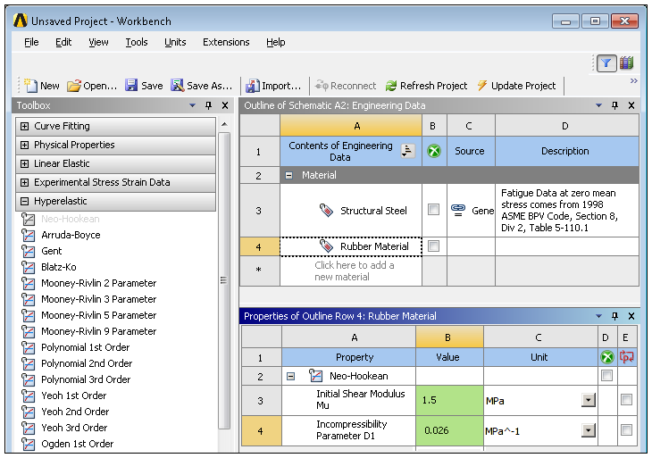
Click the toolbar button to return to the Project Schematic.
Attach Geometry.
In the Static Structural schematic, right-click the Geometry cell and choose Import Geometry>Browse.
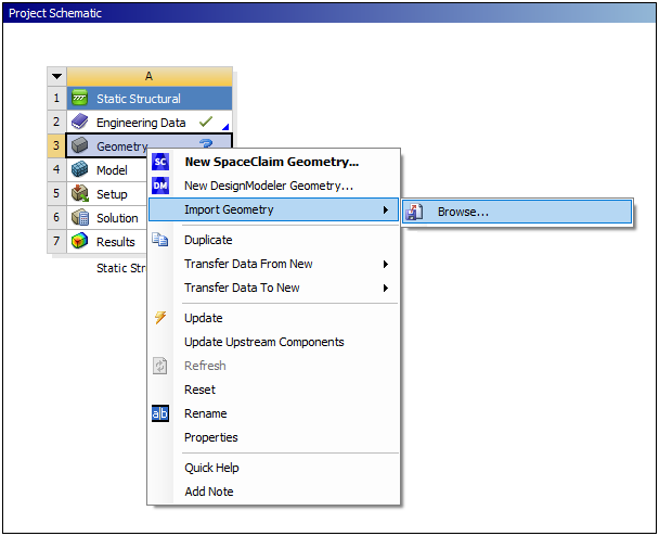
Browse to the proper folder location and open the file BootSeal_Cylinder.agdb. This file is available here on the Ansys customer site.
Important: This input file already includes predefined Named Selections that you will use for scoping.
The steps to define the model in preparation for analysis are described below. You may wish to refer to the Modeling section of Chapter 26: Nonlinear Analysis of a Rubber Boot Seal in the Mechanical APDL Technology Showcase: Example Problems to see the steps taken in the Mechanical APDL Application.
Launch Mechanical by right-clicking the Model cell and then choosing . (Tip: You can also double-click the Model cell to launch Mechanical).
Define Unit System: from the Home tab, select from the Units drop-down menu. Also select as the angular unit.
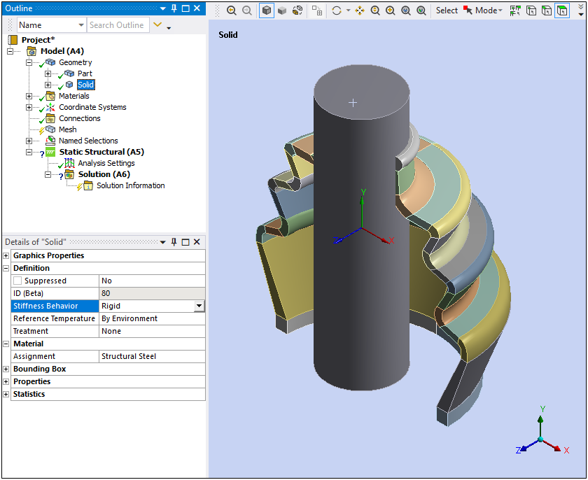
Define stiffness behavior: expand the Geometry folder and select the Solid Body object. Set the Stiffness Behavior to .
In the Geometry folder, select the Part geometry object. In the Details under the Material category, open the Assignment property fly-out menu and select .
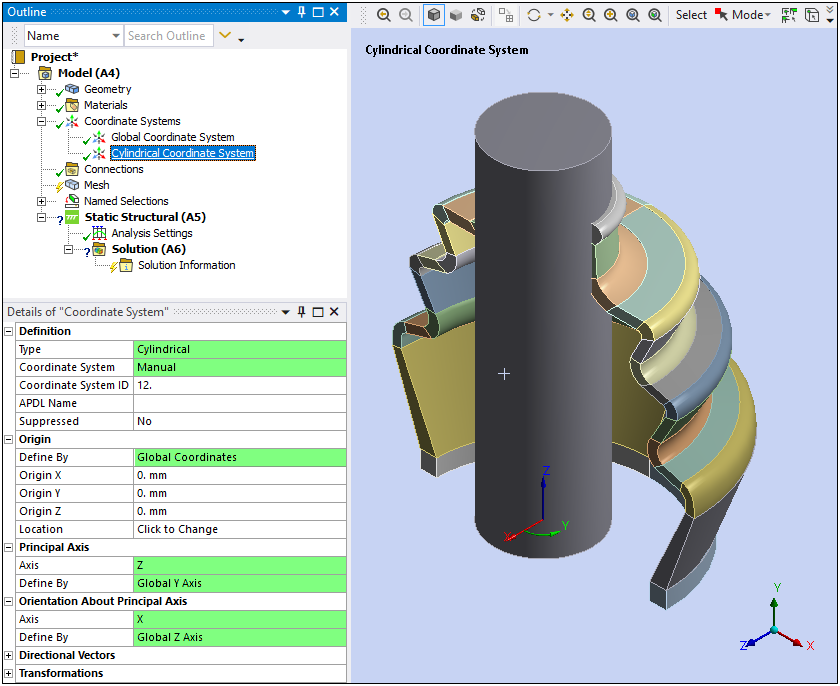
Create a Cylindrical Coordinate System: Right-click the Coordinate Systems folder and select . Highlight the new Coordinate System object, right-click, and rename it to "Cylindrical Coordinate System".
Specify properties of the Cylindrical Coordinate System:
Under the Details view Definition category, change Type to and Coordinate System to .
Under the Origin group, change the Define By property to .
Under Principal Axis select as the Axis value and set the Define By property to .
Under Orientation About Principal Axis, select as the Axis value and select for the Define By property.
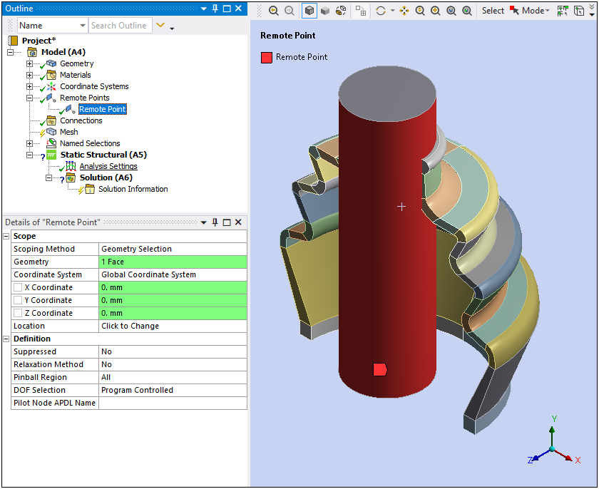
Insert Remote Point: Right-click the Model object and select > .
In Details view, scope the Geometry to the cylinder’s exterior surface, set X Coordinate, Y Coordinate, and Z Coordinate to
0.
Insert a Connection Group and Manual Contacts:
Highlight the Connections folder, right-click, and select .
Right-click the Connections Group object and select >. Notice that the Connection Group is automatically renamed to Contacts and that the new contact region requires definition.
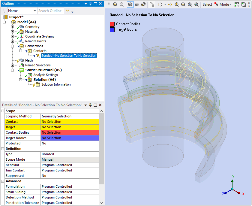
Create a Rigid-Flexible contact between the rubber boot and cylindrical shaft by defining the following Details view properties of the newly added Bonded-No Selection To No Selection.
Scoping Method set to .
Contact set to from drop-down list of Named Selections.
Target set to from drop-down list of Named Selections.
Type set to .
Frictional Coefficient Value equal to
0.2.Set Behavior set to .
Detection Method set to .
Interface Treatment set to .
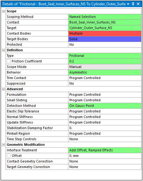
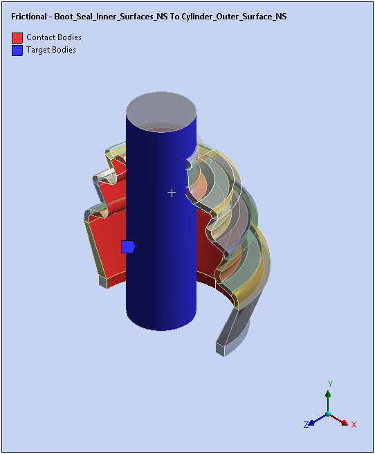
Note: The name of the contact, Bonded-No Selection To No Selection, is automatically renamed to Frictional - Boot_Seal_Inner_Surfaces_NS To Cylinder_Outer_Surface_NS.
Right-click the Contacts folder object and select . Set Contact at inner surface of the boot seal. In details view of the newly added Bonded-No Selection To No Selection, change the following properties:
Scope set to .
Contact and Target set to .
Type set to .
Frictional Coefficient value equal to
0.2.Detection Method set to Nodal-Projected Normal From Contact.
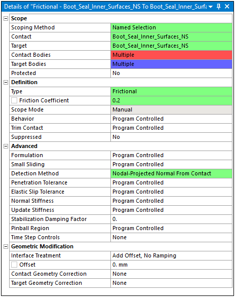
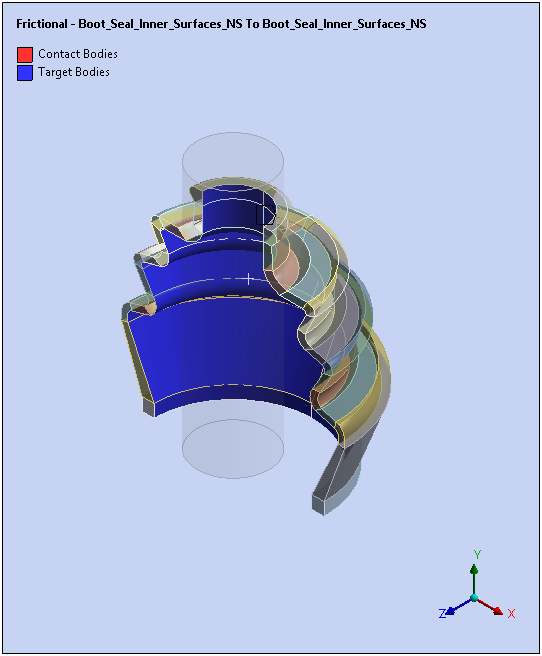
Note: The Bonded-No Selection To No Selection is automatically renamed to Frictional - Boot_Seal_Inner_Surfaces_NS To Boot_Seal_Inner_Surfaces_NS.
Right-click the Contacts folder object and select . Set Contact at inner surface of the boot seal. Self Contact at outer surface of the boot seal. In details view of the newly added , specify the following properties:
Scoping Method set to .
Contact and Target set to .
Type set to .
Frictional Coefficient Value equal to
0.2.Detection Method set to .
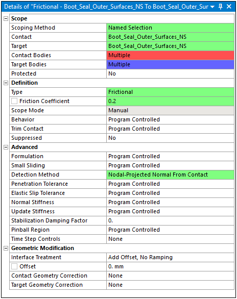
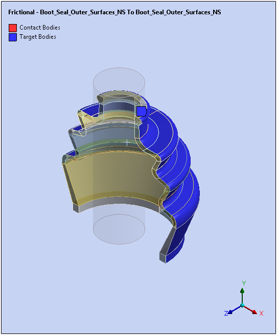
Note: Bonded-No Selection To No Selection is automatically renamed to Frictional - Boot_Seal_Outer_Surfaces_NS To Boot_Seal_Outer_Surfaces_NS.
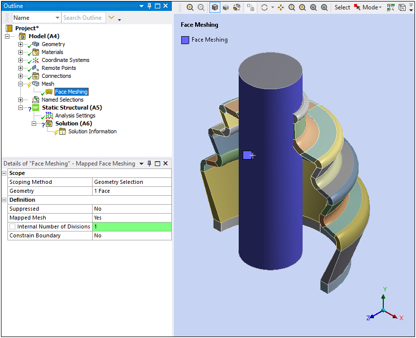
Add Mesh Controls:
Select the Mesh object and set the Element Order property to .
Right-click the Mesh object and select > . Scope the Geometry property to the exterior surface of the cylinder and set the Internal Number of Divisions property to .
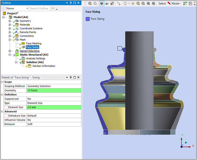
Right-click the Mesh object and select > . Scope the Geometry property to the (15) surfaces highlighted below. Set the property to .
The problem is solved in three load steps, which include:
Initial interference between the cylinder and boot.
Vertical displacement of the cylinder (axial compression in the rubber boot).
Rotation of the cylinder (bending of the rubber boot).
Load steps are specified through the properties of the Analysis Settings object.
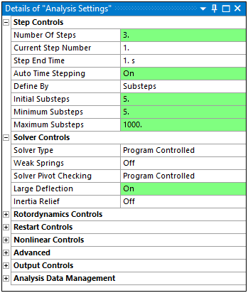
Highlight the Analysis Settings object.
Define the following properties:
Number of Steps equals
3.Auto Time Stepping set to (from Program Controlled).
Define By set to .
Initial Substeps and Minimum Substeps set to
5.Maximum Substeps set to
1000.Large Deflection set to .
For the second load step, define the properties as follows:
Current Step Number to
2.Auto Time Stepping set to (from Program Controlled).
Initial Substeps and Minimum Substeps set to
10.Maximum Substeps set to
1000.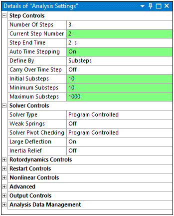
For the third load step, define the properties as follows:
Current Step Number to
3.Auto Time Stepping set to (from ).
Initial Substeps and Minimum Substeps set to
20.Maximum Substeps set to
1000.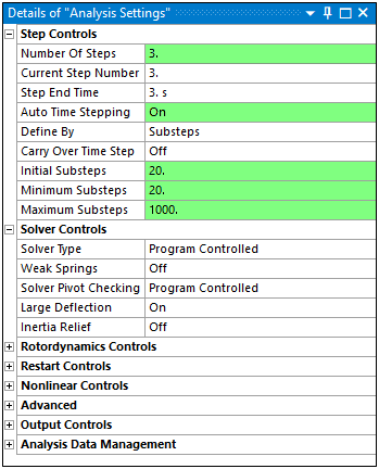
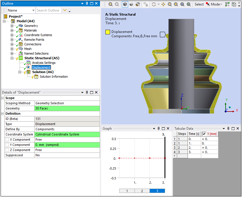
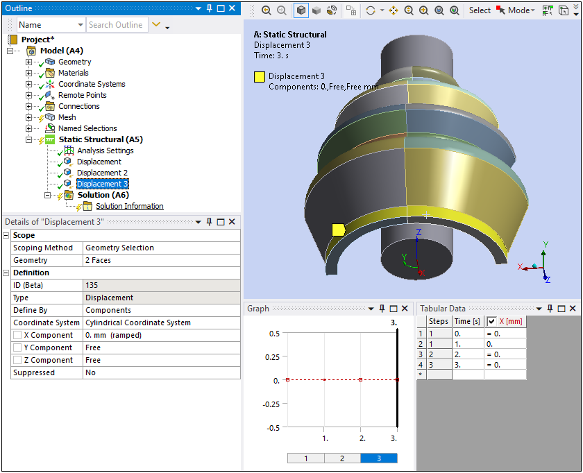
The model is constrained at the symmetry plane by restricting the out-of-plane rotation (in Cylindrical Coordinate System). The bottom portion of the rubber boot is restricted in axial (Y axis) and radial directions (in Cylindrical Coordinate System).
Right-click the Static Structural (A5) object and select .
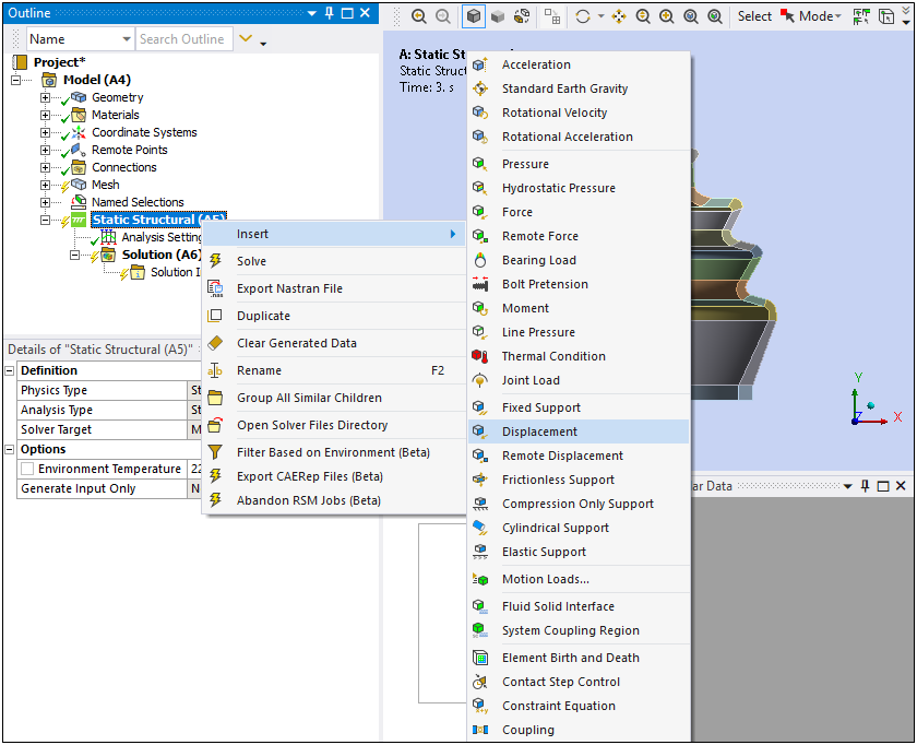
Select the faces (press the Ctrl key and then select each face) of the rubber boot seal as illustrated below.
Set the Coordinate System property to and the Y Component property to
0.
Select the faces illustrated here and insert another . Set the Y Component to
0(Coordinate System should equal ).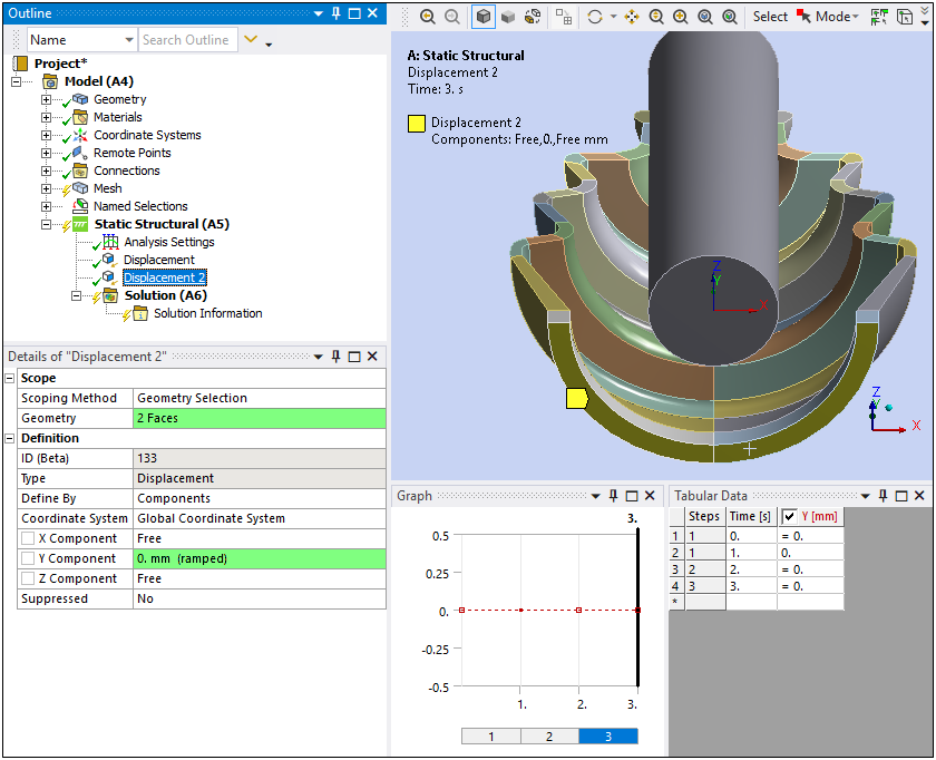
Insert another scoped as illustrated here and set the Coordinate System property to and the X Component property to
0.
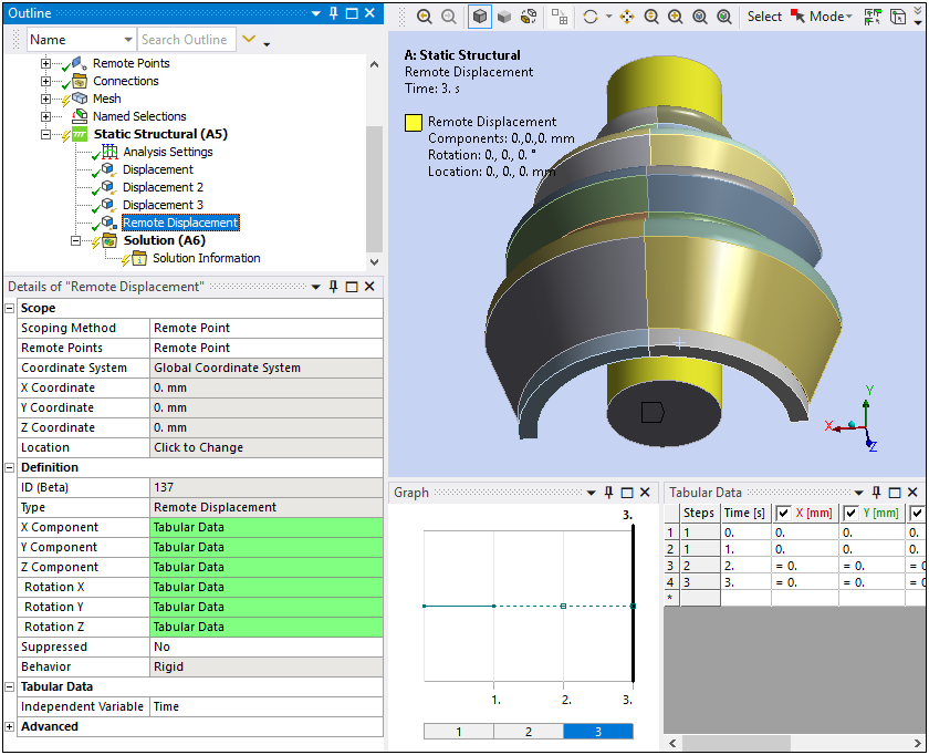
Insert a .
Set the Scoping Method of the Remote Displacement to .
Select the created earlier (only option) for the Remote Points property.
Change the X Component, Y Component, Z Component, Rotation X, Rotation Y, and Rotation Z properties to as illustrated below.
Specify the following Tabular Data values:
Y value for Step 2 and Step 3 as
-10mm.RZ value for Step 3 as
0.55[rad].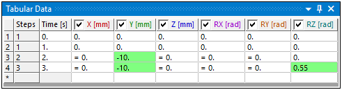
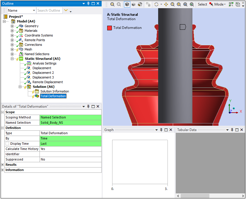
Insert a result from the Solution object.
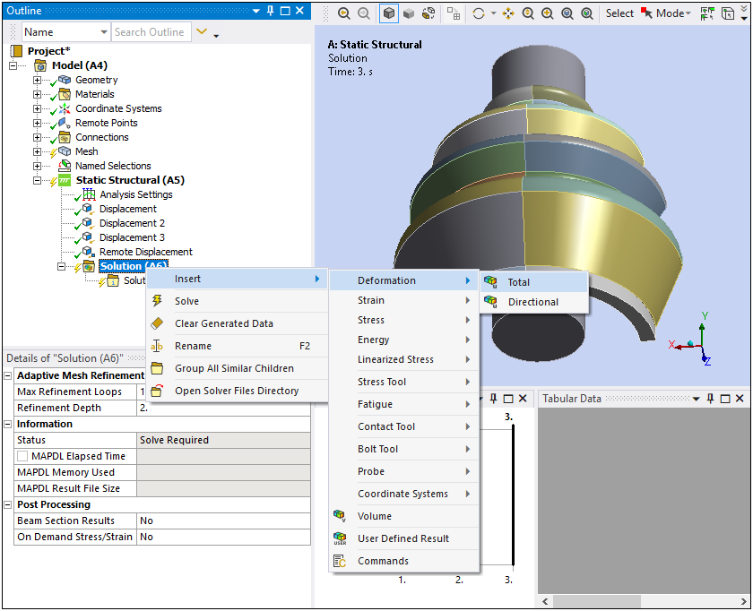
Specify the Scoping Method as Named Selection and select as the Named Selection.
As needed, set the By property to and the Display Time property to .
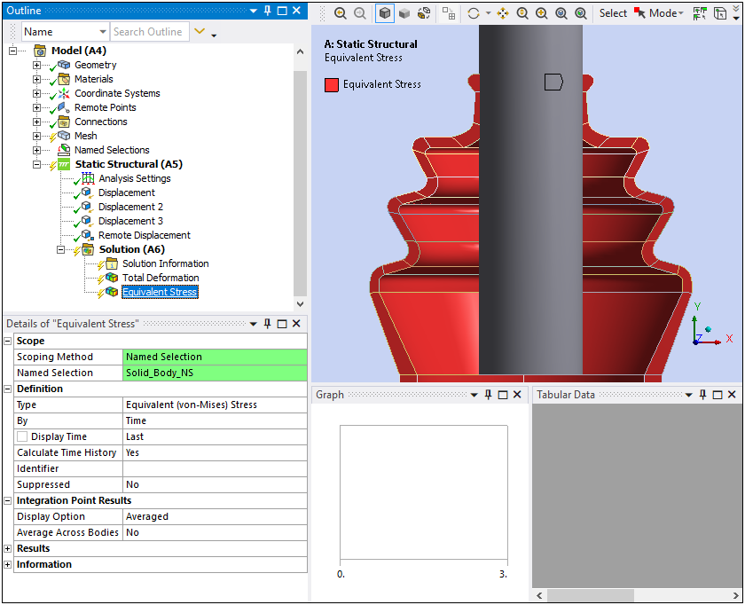
Insert a result from the Solution object.
Specify the Scoping Method to Named Selection and select as the Named Selection.
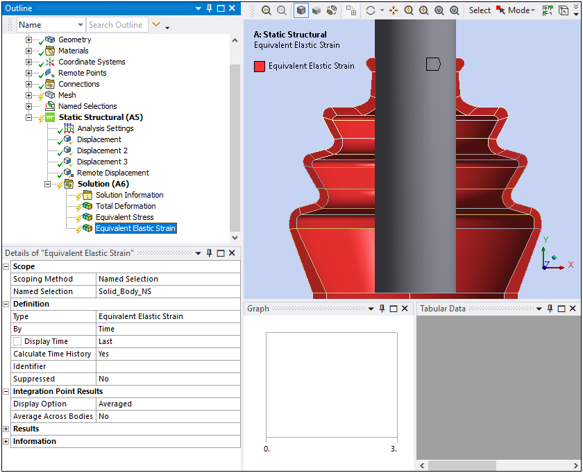
Insert a result from the Solution object.
Specify the Scoping Method to Named Selection and select as the Named Selection.
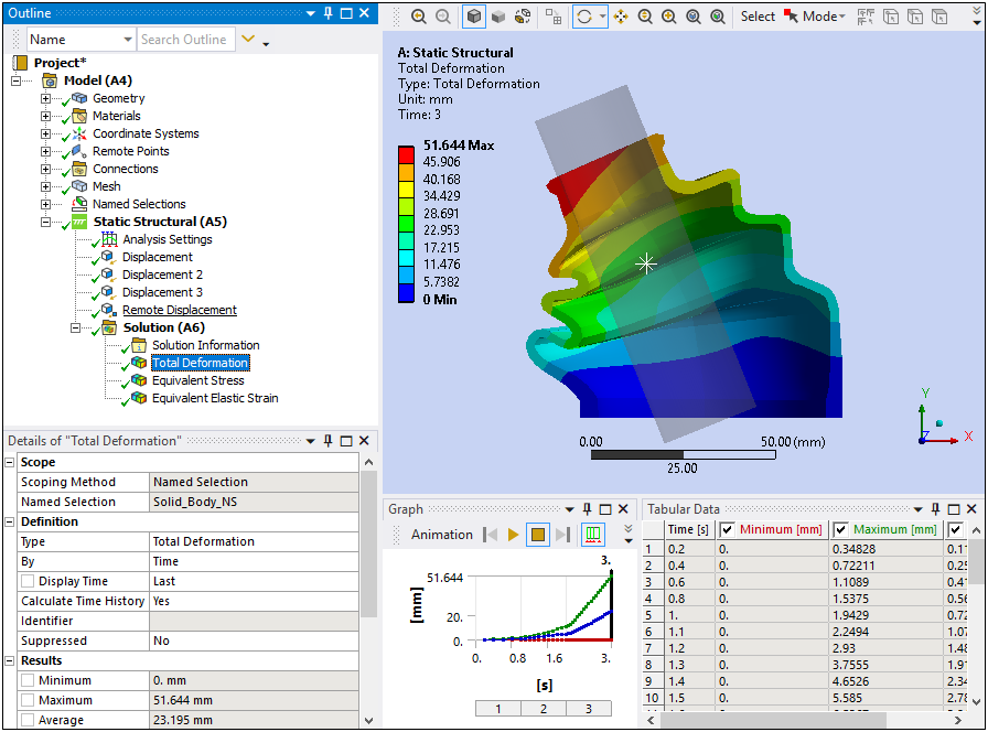
Click the button.
Note:
The default mesh settings keep mid-side nodes in the SOLID186 elements (See Solution Information). You can drop mid-side nodes in the Mesh object Details view under the Advanced group. This allows you to mesh and solve faster with lower order elements.
Although very close, the mesh generated in this example may be slightly different than the one generated in Chapter 26: Nonlinear Analysis of a Rubber Boot Seal in the Mechanical APDL Technology Showcase: Example Problems.
The solution objects should appear as illustrated below. You can ignore any warning messages.
For a more detailed examination and explanation of the results, see the Results and Discussion section of Chapter 26: Nonlinear Analysis of a Rubber Boot Seal in the Mechanical APDL Technology Showcase: Example Problems.
Total Deformation at Maximum Shaft Angle
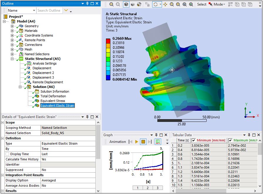
Equivalent Elastic Strain at Maximum Shaft Angle (at the end of 3 seconds)
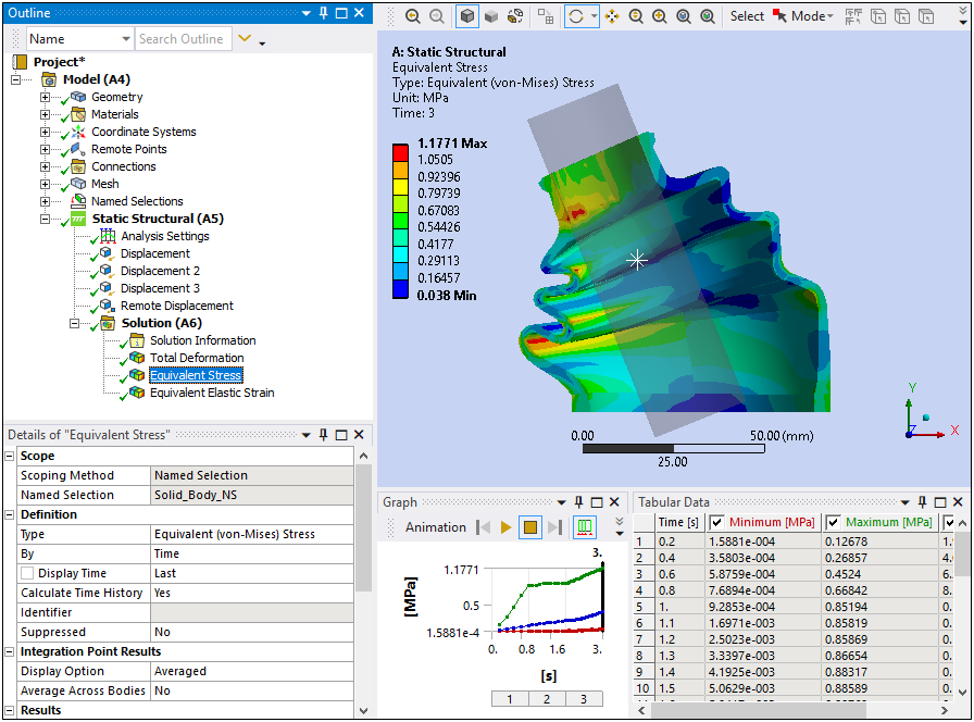
Equivalent Stress (Von-Mises Stress) at Maximum Shaft Angle
Congratulations! You have completed the tutorial.