


This example problem demonstrates the use of a Rigid Dynamics analysis to examine the kinematic behavior of an actuator after a moment force is applied to the flywheel.
| Analysis Type | Rigid Dynamics |
| Features Demonstrated | Joints, joint loads, springs, coordinate system definition, body view, joint probes |
| Licenses Required | Ansys Mechanical Premium/Enterprise/Enterprise PrepPost |
| Help Resources | Rigid Dynamics Analysis, Revolute Joint, Translational Joint |
| Tutorial Files | actuator.agdb |
This tutorial guides you through the following topics:
Start by creating a Rigid Dynamics analysis system and importing geometry.
Start Ansys Workbench.
In the Workbench Project page, drag a Rigid Dynamics system from the Toolbox into the Project Schematic.
Right-click the Geometry cell of the Rigid Dynamics system, and select >.
Browse to open the Actuator.agdb file. This file is available here on the Ansys customer site. A check mark appears next to the Geometry cell in the Project Schematic when the geometry is loaded.
Prepare the Analysis in the Mechanical Application
In the Rigid Dynamics system schematic, right-click the Model cell, and select Edit. The Mechanical Application opens and displays the model.
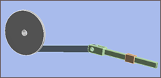
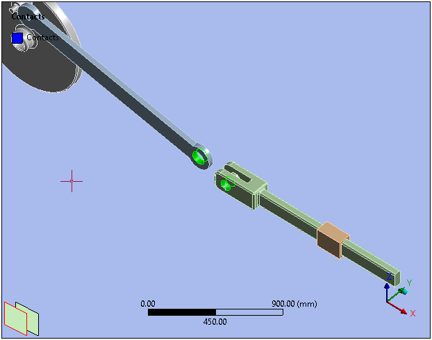
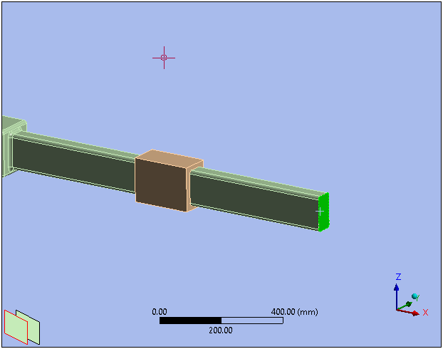
The actuator mechanism model consists of four parts: (from left to right) the drive, link, actuator, and guide.
From the Home tab, open the drop-down menu and select .
Note: Stiffness behavior for all geometries are rigid by default.
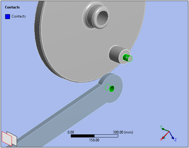
Rigid dynamics models use joints to describe the relationships between parts in an assembly. As such, the surface-to-surface contacts that were transferred from the geometry model are not needed in this case. To remove surface-to-surface contact:
Expand the Connections branch in the Outline, then expand the Contacts branch. Highlight all of the Contact Regions in the Contacts branch.
Right-click the highlighted contact regions, then select .
Note that this step is not needed if your Mechanical options are configured so that automatic contact detection is not performed upon attachment.
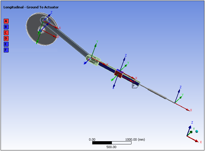
Joints will be defined in the model from left to right as shown below, using Body-Ground and Body-Body joints as needed to solve the model.
Prior to defining joints, it is useful to select the button in the Connections toolbar. The button splits the graphics window into three sections: the main window, the reference body window, and the mobile body window. Each window can be manipulated independently. This makes it easier to select desired regions on the model when scoping joints.
To define joints:
Select the drive pin face and link center hole face as shown below, then select > from the Joint group on the Connections Context tab.
Note: In the illustration above, the Explode feature of the Display tab was used to separate parts for easy selection.
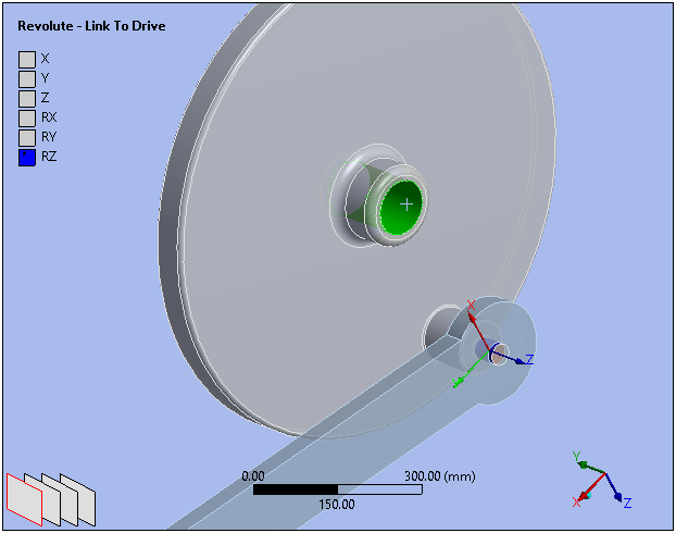
Select the drive center hole face as shown below, then select > from the Joint group on the Connections Context tab.
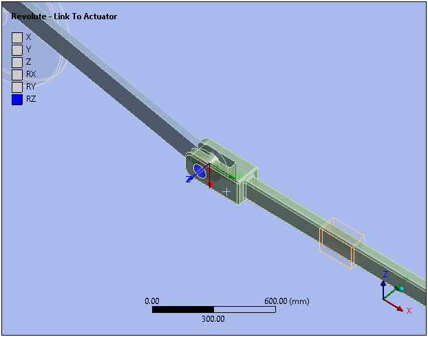
Select the link face and actuator center hole face as shown below, then select > from the Joint group on the Connections Context tab.
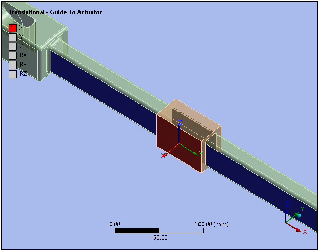
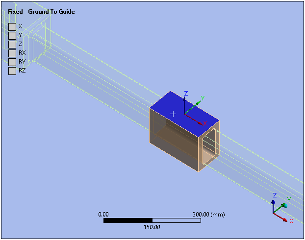
Select the actuator face and the guide face as shown below, then select > from the Joint group on the Connections Context tab.
Select the guide top face as shown below, then select > from the Joint group on the Connections Context tab.
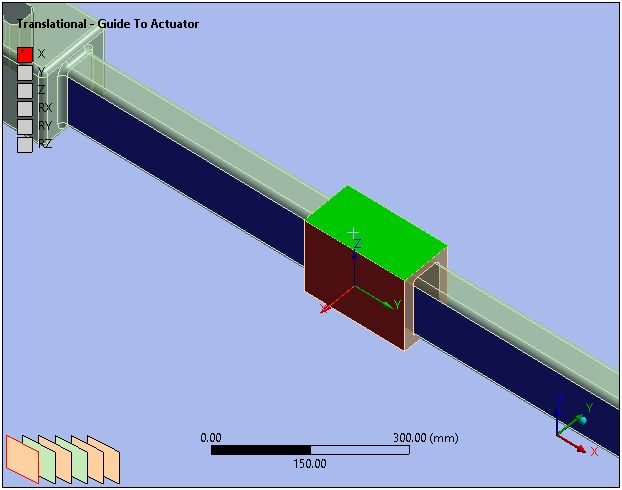
The coordinate systems for each new joint must be properly defined to ensure correct joint motion. Realign each joint coordinate system so that they match the corresponding systems pictured in Define Joints. To specify a joint coordinate system:
In the Outline, highlight a joint in the Joints branch.
In the joint Details view, click the Coordinate System field. The property becomes active.
Click the axis you want to change (X, Y, or Z). All six directions become visible as shown below.
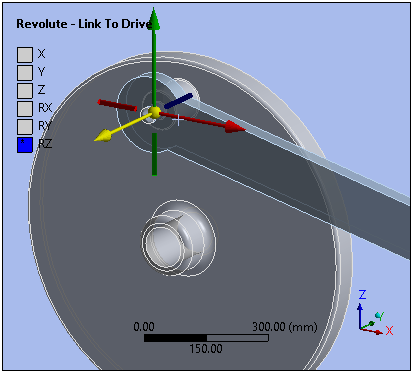
Click the desired new axis to realign the joint coordinate system.
Select in the Details view once the desired alignment is achieved.
A local coordinate system must be created. This will be used to define a spring which will be added to the actuator.
Right-click the Coordinate Systems branch in the Outline, then select >.
Right-click the new coordinate system, then select . Enter
Spring_fixas the name.In the Details for the
Spring_fixCoordinate System, define the Origin fields using the values shown below: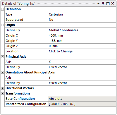
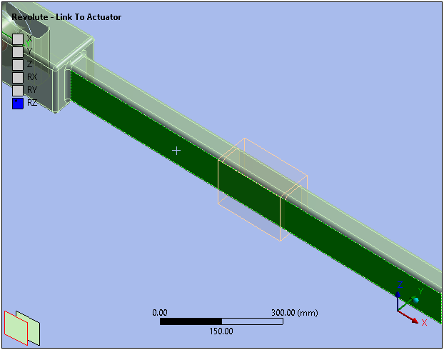
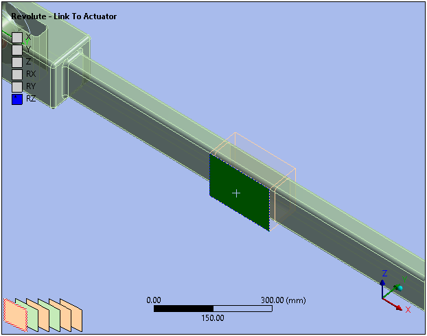
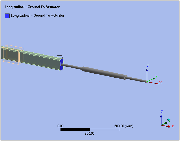
Select the bottom face of the actuator as shown below, then open the Spring drop-down menu from the Connect group of the Connections Context tab and select .
In the Reference section of the spring Details view, set the Coordinate System to
Spring_fix.In the Definition section of the spring Details view, specify:
Longitudinal Stiffness = 0.005 N/mm Longitudinal Damping = 0.01 N*s/mm 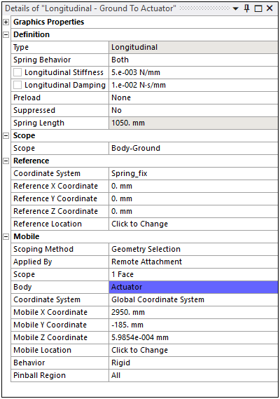
To define the length of the analysis:
Select the Analysis Settings branch in the Outline.
In the Analysis Settings Details, specify the Step End Time property equal to 60 s.
A joint load must be defined to apply a kinematic driving condition to the joint object. To define a Joint Load:
Right-click the Transient object in the Outline and select Insert>Joint Load.
For the Joint Load, specify the following properties:
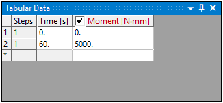
Joint = Type = Magnitude = Specify as Tabular (Time) Graph and Tabular Data windows will appear.
In the Tabular Data window, specify that Moment = 5000 at Time = 60, as shown below.
Select Solution object in the Outline, then open the Deformation drop-down menu of the Results group on the Context tab and select Total.
In the Outline, click and drag and drop the Revolute - Link to Actuator joint onto the Solution object. This automatically creates a Joint Probe under the Solution object.
This is a shortcut for creating a joint probe that is already scoped to the joint in question to find the forces acting on this joint, the default settings in the details of the joint probe are used.
Click the Solve button in the main toolbar.
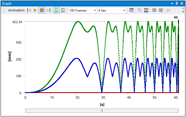
After the solution is complete, select Total Deformation result. A timeline animation of max/min deformation vs. time appears in the Graph window.
In the Graph window, select the animation option. Specify 100 frames and 4 seconds, as shown below. (These values have been chosen for efficiency purposes, but they can be adjusted to user preference.)
Click the button to view the animation.
Select the Joint Probe object in the Outline.
Specify the X Axis option in the Result Selection property.
Right-click the Joint Probe object, and select Evaluate All Results.
The results from the analysis show that the spring-based actuator is adding energy in to the system that is reducing the cycle time.
Congratulations! You have completed the tutorial.