


This tutorial demonstrates the use of cyclic symmetry analysis features in Mechanical to study a sector of a rotor and brake assembly in frictional contact.
| Analysis Type | Cyclic Symmetry |
| Features Demonstrated | Cyclic region, Named Selections based on criteria, thermal steady-state analysis with cyclic symmetry, static structural analysis with cyclic symmetry, modal analysis with cyclic symmetry, generation of restart points, modal analysis with nonlinear pre-stress (linear perturbation) |
| Licenses Required | Ansys Mechanical Premium/Enterprise/Enterprise PrepPost |
| Help Resources | Analysis Settings for Cyclic Symmetry in a Modal Analysis |
| Tutorial Files | Rotor_Brake.agdb |
This tutorial guides you through the following topics:
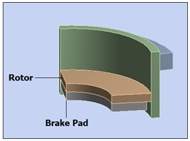
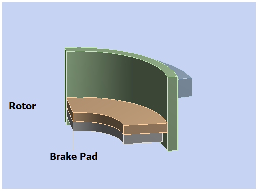
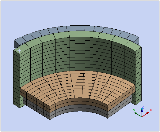
A quarter sector model of a rotor and brake assembly in frictional contact is shown below. With increased loading of the brake, the contact status between the pad and the rotor changes from near, to sliding, to sticking. Each of these contact states affects the natural frequencies and resulting mode shapes of the assembly. Three pre-stress modal analyses are used to verify this phenomenon.
Note: The procedural steps in this tutorial assume that you are familiar with basic navigation techniques within the Mechanical application. If you are new to using the application, consider running the tutorial: Steady-State and Transient Thermal Analysis of a Circuit Board before attempting to run this tutorial.
We will tour the different analysis systems that can leverage cyclic symmetry functionality. These are thermal, static structural and modal analyses:
A steady-state thermal analysis will be used to calculate the temperature distribution for the evaluation of any temperature-dependent material properties or thermal expansions in subsequent analyses.
A nonlinear static structural analysis is configured to represent the mechanical loading of the brake onto the rotor. Nonlinearities from large deformation and changes in contact status are included.
Modal analyses, each at different stages of frictional contact status, are established to compare the free vibration responses of the model.
Create the analysis systems.
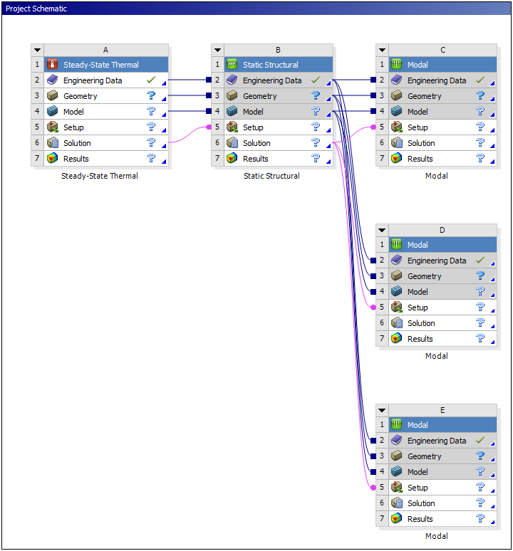
You need to establish a Steady-State Thermal analysis that is linked to a Static Structural analysis, then establish three Modal analyses that are linked to the Static Structural analysis.
Start Ansys Workbench.
From the Toolbox, drag a Steady-State Thermal system onto the Project Schematic.
From the Toolbox, drag and drop a Static Structural system onto the Steady-State Thermal system such that Cells 2, 3, 4, and 6 are highlighted in red.
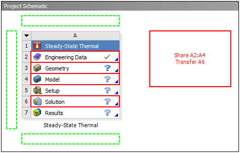
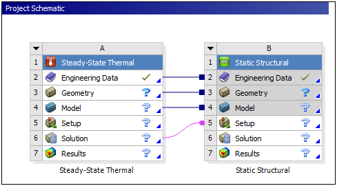
The systems should appear as follows:
To measure the free vibration response, go to the Toolbox, drag and drop a Modal system onto the Static Structural system such that cells 2, 3, 4, and 6 are highlighted in red.
Repeat the above step two more times to complete adding the remaining analysis systems. The layout of the analysis systems and interconnections in the Project Schematic should appear as shown below.
Attach geometry.
Right-click the Geometry cell of the Steady-State Thermal system and select Import Geometry.
Browse to open the file Rotor_Brake.agdb. This file is available here on the Ansys customer site.
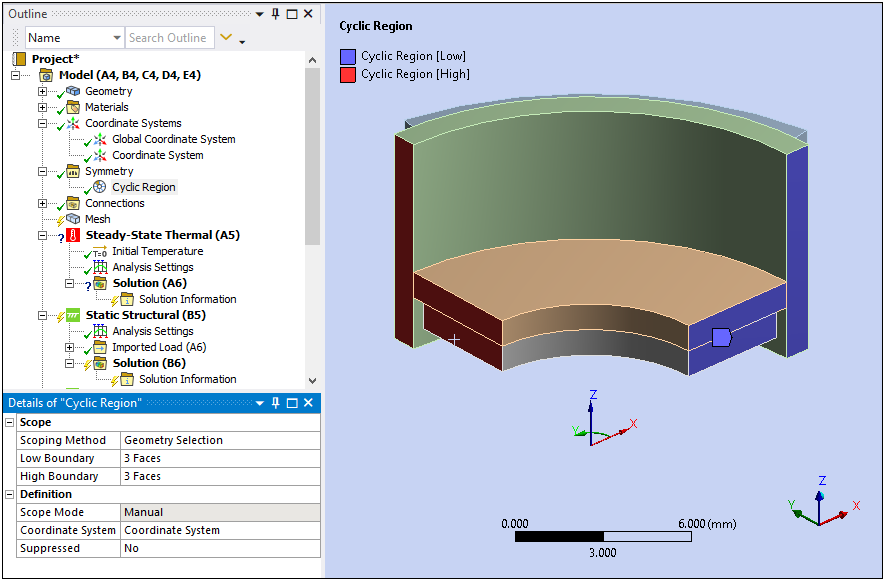
We now specify the cyclic symmetry for our quarter sector model (N = 4, 90 degrees) and prepare other general aspects of modeling in the Mechanical application. To set up a cyclic symmetry analysis, Mechanical uses a Cyclic Region object. This object requires selection of the sector boundaries, together with a cylindrical coordinate system whose Z axis is collinear with the axis of symmetry, and whose Y axis distinguishes the low and high boundaries.
Launch Mechanical and set unit systems.
In the Steady-State Thermal schematic, right-click the Model cell, and then choose Edit. The application opens and displays the model.
From the Tools group on the Home tab, open the Units drop-down menu and select .
Define the Coordinate System to specify the axis of symmetry.
Right-click the Coordinate Systems object in the Outline and select .
In the Details view of the newly-created Coordinate System, set the Type property to Cylindrical and the Define By property to Global Coordinates.
Define the Cyclic Region.
Right-click the Model object and select > .
Right-click Symmetry and select > . The direction of the Y-axis should be compatible with the selection of the low and high boundaries. The low boundary is designated as the one with a lower value of Y or azimuth.
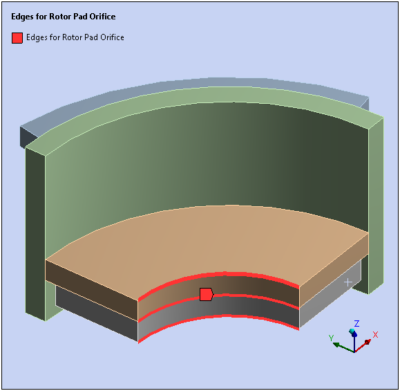
Select the three faces that have lower azimuth for the low boundary as illustrated in blue in the image below.
Select the three matching faces on the opposite end of the sector for the high boundary as illustrated in red in the image below.
Define Connections. Frictional contact exists between the rotor and brake pad, whereas bonded contact exists between the wall and the rotor.
Expand the Connections folder in the tree, then expand the Contacts folder. Within the Contacts folder, two contact regions were automatically detected: Contact Region and Contact Region 2.
Right-click the Contacts folder and select . The contact region names automatically change to Bonded - Pad to Rotor and Bonded - Blade to Wall respectively.
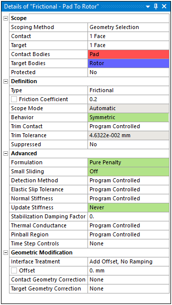
Highlight Bonded - Pad to Rotor and in the Details view, set Type to Frictional. Note that the name of the object changes accordingly.
In the Friction Coefficient field, type 0.2 and press Enter.
Note: For higher values of contact friction coefficient a damped modal analysis would be needed. At a level of 0.2 damping effects are being neglected.
Verify that the following additional properties are specified as shown.
We’ll use mesh controls to obtain a mesh of regular hexahedral elements. The Cyclic Region object guarantees that matching meshes are generated on the low and high boundaries of the cyclic sector.
Taking advantage of the shape and dimensions of the model, use Named Selections to choose the edge selections for each mesh control.
Mesh control: Element Size on Pad-Wall-Rotor:
Create a Named Selection for this Mesh Control.
Right-click the Model object and select > .
Highlight the Selection object and set the Scoping Method property to Worksheet.
Program the Worksheet, as shown below, to select the edges at 90 degrees of azimuth in the cylindrical coordinate system, keeping those in the z-axis range [1 mm, 6 mm] (to remove the thickness of the wall). To add rows to the Worksheet, right-click in the table and select the option.
Click the Generate button. The Geometry property should display 11 Edges.
Rename the object to Edges for Wall Rotor Pad Sector Boundary. The selection should display as follows:
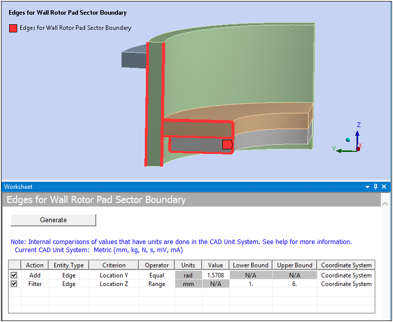
Tip: It may be useful to undock the Worksheet window and tile it with the Geometry view as shown above.
Insert a Mesh Sizing control.
Right-click the Mesh object and select > .
Set Scoping Method to Named Selection.
Choose the Named Selection defined in the previous step: Edges for Wall Rotor Pad Sector Boundary.
Set the Element Size property to 0.5 mm.
Set the Behavior property to Soft (default).
Mesh control: Number of Divisions on Pad-Rotor:
Create a Named Selection to pick the circular edges in the orifice of the pad and rotor.
This Named Selection will pick the circular edges in the orifice of the pad and rotor, which is within a radius of 5 mm.
Right-click Model and choose.
Highlight the Selection object, and set Scoping Method to Worksheet.
Rename the object to Edges for Rotor Pad Orifice.
Program the Worksheet, as shown below.
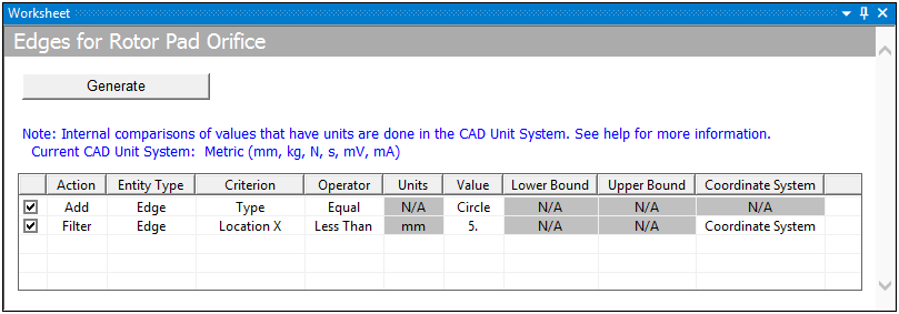
Click the Generate button. The Geometry property should display 4 Edges.
Insert a Mesh Sizing Control as before to select this Named Selection.
Right-click the Mesh object and select > .
Set Scoping Method to Named Selection.
Select the Named Selection defined in the previous step: Edges for Rotor Pad Orifice.
Set the Type property to Number of Divisions and specify the Number of Divisions property to .
Set Behavior property to Hard.
Mesh control: Element Size on Wall-Blade
Create a Named Selection object to pick the thicknesses of the Wall and Blade.
Right-click Model and choose.
Highlight the Selection object, and set Scoping Method to Worksheet.
Rename the object to Edges for Wall Blade Thicknesses.
Specify the Worksheet as shown below.
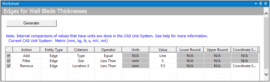
Click the Generate button. The Geometry property should display 16 Edges.
Insert a Mesh Sizing Control as before to select this Named Selection.
Right-click the Mesh object and select > .
Set the Scoping Method property to Named Selection.
Select the Named Selection defined in the previous step: Edges for Wall Blade Thicknesses.
Set the Element Size property to .
Set Behavior property to Hard.
Mesh Control: Number of Divisions on Blade - Longer Edges
Create a Named Selection object to pick the longer edges of the Blade.
Right-click the Model object and select > .
Highlight the Selection object, and set Scoping Method to Worksheet.
Rename the object to Edges for Blade.
Program the as shown below.
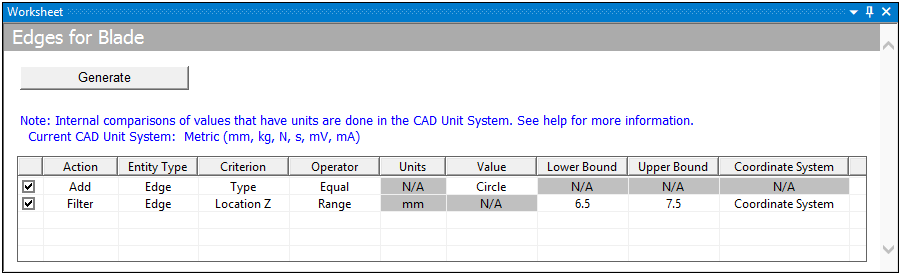
Click the Generate button. The Geometry property should display 2 Edges.
Insert a Mesh Sizing Control as before to select this Named Selection.
Right-click the Mesh object and select > .
Set the Scoping Method property to Named Selection.
Select the Named Selection defined in the previous step: Edges for Blade.
Set the Type property to Number of Divisions and set the Number of Divisions property to .
Set the Behavior property to Hard.
Mesh Control: Number of Divisions on Blade - Shorter Edges
Create a Named Selection object to pick the shorter edges of the Blade.
Right-click the Model object and select > .
Highlight the Selection object, and set the Scoping Method property to Worksheet.
Rename the object to Edges for Blade 2.
Specify the Worksheet as shown below.
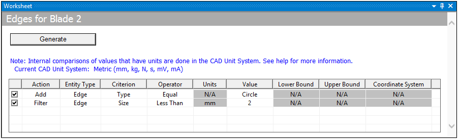
Click the Generate button. The Geometry property should display 2 Edges.
Insert a Mesh Sizing Control as before to select this Named Selection.
Right-click the Mesh object and select > .
Set Scoping Method to Named Selection.
Select the Named Selection defined in the previous step: Edges for Blade 2.
Set the Type to Number of Divisions and set the Number of Divisions property to (default).
Set the Behavior property to Hard.
Mesh Control: Method on Pad-Rotor-Wall-Blade
Insert a Sweep Method control.
Right-click the Mesh object and select > .
Select all the bodies of the model by right-clicking in the Geometry window, selecting , and then selecting the button of the Geometry property in the Details. The key combination Ctrl+A selects all bodies.
In the Details, set the Method property to Sweep.
Set the Free Face Mesh Type property to All Quad.
Generate the Mesh
For convenience, select all six mesh controls defined, right-click, and select .
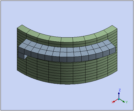
Right-click the Mesh object and select Generate Mesh. The mesh should appear as shown below:
We now proceed to define the boundary conditions for a thermal analysis featuring cyclic symmetry. Thermal boundary conditions are prescribed throughout the model while steering clear of the faces comprising the sector boundaries since temperature constraints are already implied there.
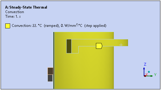
Define a convection interface.
Right-click the Steady-State Thermal object and select > .
Select the outer faces of the Wall and the Blade as shown in the figure ().
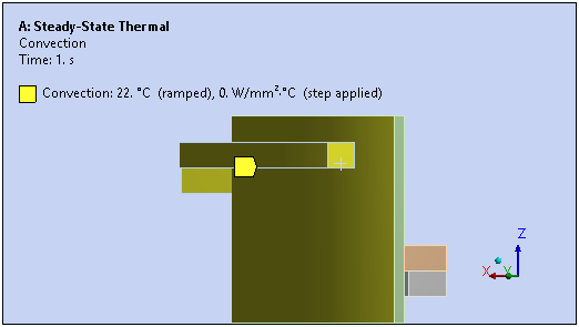
Specify a Film Coefficient of air by right-clicking on the property and choosing Import Temperature Dependent upon which you choose Stagnant Air - Simplified Case.
Insulate the upper and lower faces of the Wall.
Select the upper and lower faces of the Wall, then right-click and choose.
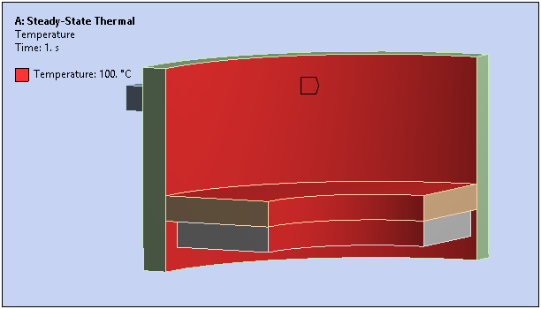
Apply a temperature load to the Pad and Rotor.
Select the remaining faces on the assembly on the Pad and the Rotor, then right-click and choose. Exclude any faces on the sector boundaries or in the frictional contact.
Type 100°C as the Magnitude and press Enter.
Solve and review the temperature distribution.
Right-click the Solution object of the Steady-State Thermal analysis and select > > .
Solve the steady-state thermal analysis.
Review the temperature result by highlighting the Temperature result object.
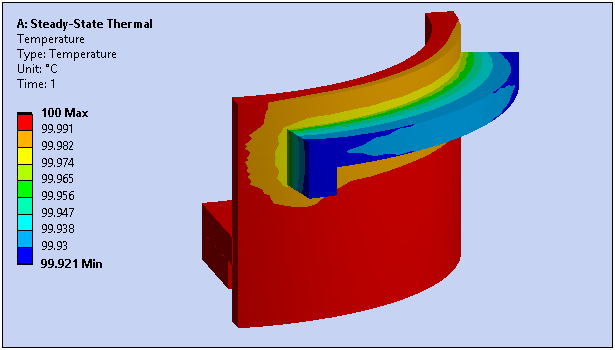
Note: Although insignificant in this model, temperature variations and their effect on the structural material properties are generally important to the formulation of physically accurate models.
In this analysis, the brake is loaded onto the rotor in a single load step. The contact status is monitored at various stages of loading and three points are selected as pre-stress conditions for subsequent modal analyses. Because both contact and geometric nonlinearities are present, each pre-stress condition will present a different effective stiffness matrix to its corresponding modal analysis.
The solver uses restart points, generated in the static analysis, to record the snapshot of the nonlinear tangent stiffness matrices and transfers them into the subsequent linear systems. This technique is referred to as Linear Perturbation.
Apply the pressure and boundary conditions to engage the brake pad into the rotor.
Select the bottom face of the Pad as shown below. Right-click the Static Structural object in the tree and choose Insert> Pressure.
In the Details view, open the Magnitude flyout menu, choose Function, and specify the entry:
=time*time*4000. Press Enter. This represents a quadratic function reaching 4000 MPa by the end of the load step.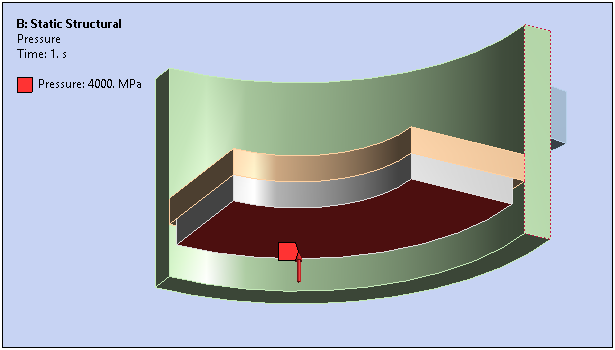
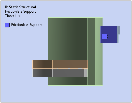
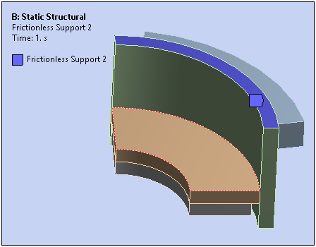
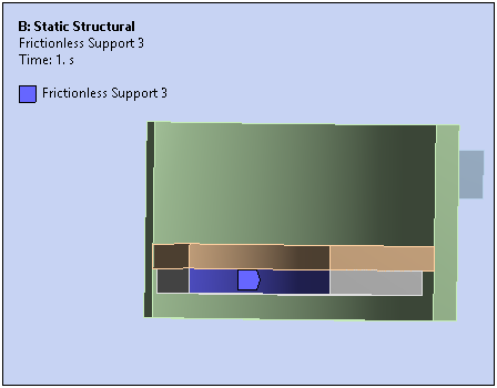
Set up the frictionless supports on the faces of Blade, Wall and Pad as shown below.
Configure the Analysis Settings.
Set Auto Time Stepping to On.
Set Define By to Substeps.
Set Initial Substeps to 30.
Set Minimum Substeps to 10.
Set Maximum Substeps to 30.
Set Large Deflection to On to activate geometric nonlinearities.
To ensure that Restart Points are generated, under Restart Controls, set Generate Restart Points to Manual, and set the Load Steps, Substeps, and Maximum Points to Save Per Step properties to All.
Proceed to solve the model using the standard procedure.
Reviewing the contact status changes during the course of the load application
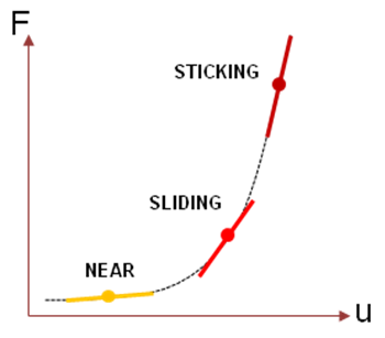
The contact status will change with increasing loads from Near, to Sliding, to Sticking. A status change from Near to Sliding reflects the engagement of contact impenetrability conditions (normal direction). A change from Sliding to Sticking, reflects additional engagement of contact friction conditions (tangential direction). This progression will generally reflect an increased effective stiffness in the tangent stiffness matrix, which can be illustrated by a Force-deflection curve:
To review the contact status, insert a Contact Tool from the Solution folder. To display only the contact results at the frictional contact, unselect Bonded - Wall To Blade in the Contact Tool Worksheet. Insert three different Contact Status results with display times of 0.03, 0.5 and 0.8 seconds. This should reveal the progression in contact status as shown below (from left to right):
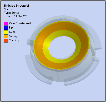
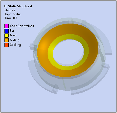
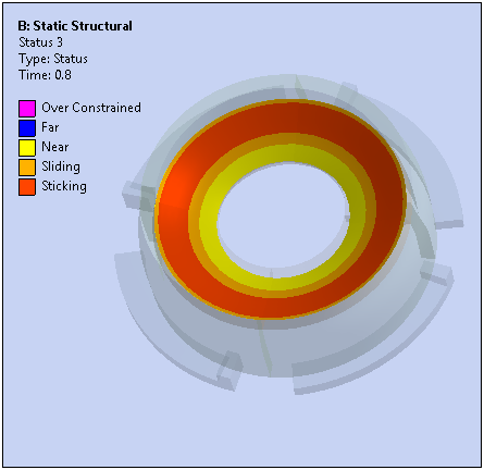
The legend for these contact status plots is as follows:
Yellow - Near
Light Orange - Sliding
Dark Orange - Sticking
There are three modal analyses to study the effect of contact status and stress stiffening on the free vibration response of the structure. Each of these will be based on a different restart point in the static structural analysis.
To see all available restart points, you can inspect the timeline graph displayed when the Analysis Settings object of the Static Structural analysis is selected after solving. Restart points are denoted as blue triangle marks atop the graph:
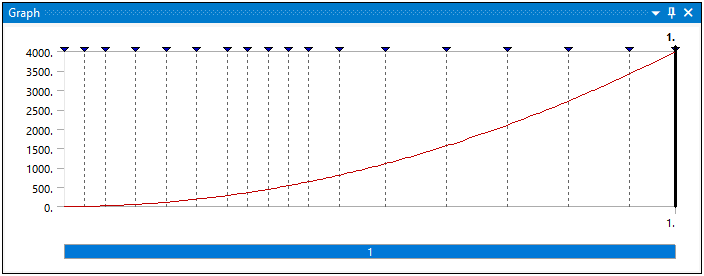
To select the restart point of interest, go to the Pre-Stress (Static Structural) object under each Modal Analysis. Make sure Pre-Stress Define By is set to Time and specify the time. The object will acknowledge the restart point in the Reported Loadstep, Reported Substep and Reported Time fields.
Configure the Modal analyses as follows:
In Modal 1 set Pre-Stress Time to 0.033 seconds.
In Modal 2 set Pre-Stress Time to 0.5 seconds.
In Modal 3 set Pre-Stress Time to 0.8 seconds.
Due to the automatic import of boundary conditions (in this case, the frictionless supports) from the static analysis, we can proceed with the solving process directly.
We'll monitor the lowest frequencies of vibration which belong to Harmonic Indices 0 (symmetric) and 2 (anti-symmetric).
Solve each Modal analysis.
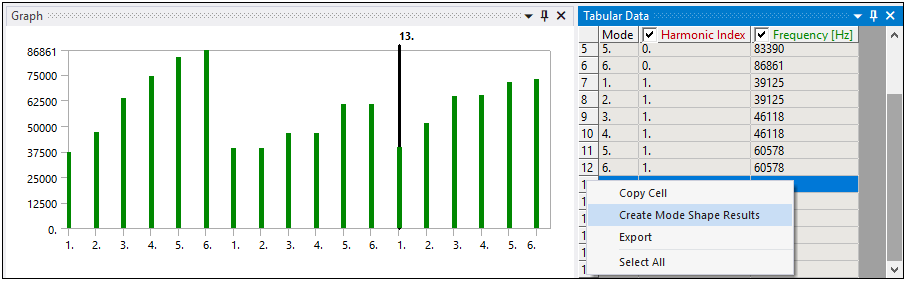
When the solutions complete, go to the Tabular Data window of each modal analysis. You can inspect the listing of modes and their frequencies. Because our structure has a symmetry of N=4, there will be three solutions, namely for Harmonic Indices 0, 1 and 2.
In the Tabular Data window of each modal analysis, select the two rows for Harmonic Index 0 - Mode 1 and Harmonic Index 2 - Mode 1. Right-click and choose .
The image below shows this view for the first Modal analysis:
An interesting alternative is to display the sorted frequency spectrum. You may review this by setting the X-Axis property to Frequency on any of the Total Deformation results in each modal analysis:
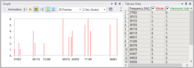
At this point, each Modal analysis should have two results for Total Deformation to inspect the first Mode of Harmonic Indices 0 and 2.
Recall the meaning of Harmonic Index solutions and how they apply to the model. Harmonic Index 0 represents the constant offset in the discrete Fourier Series representation of the model and corresponds to equal values of every transformed quantity, for example, displacements in X, Y and Z directions, in consecutive sectors. Thus deformations that are axially positive in one sector will have the same axially positive value in the next. The following picture shows, from left to right, the mode shapes for the Near, Sliding, and Sticking status at Harmonic Index 0:
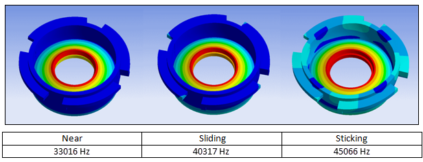
Notice how increased engagement of the frictional contact in the assembly has the effect of producing higher frequency vibrations. Also, the mode of vibration goes from being localized at the contact interface when the contact is Near, but is forced to distribute throughout the wall of the rotor as the contact sticks.
Note: You may need to specify Auto Scale on the Results toolbar so the mode shapes are plotted as shown.
Harmonic Index 2 solutions correspond to N/2 for our sector (90 degrees or N = 4). This Harmonic Index, sometimes called the asymmetric term in the Fourier Series, represents alternation of quantities in consecutive sectors. A positive axial displacement at a node in one sector becomes negative in the next, a radially outward displacement in one sector will become inward in the next, and so on. The following are the results for the first mode of this Harmonic Index:
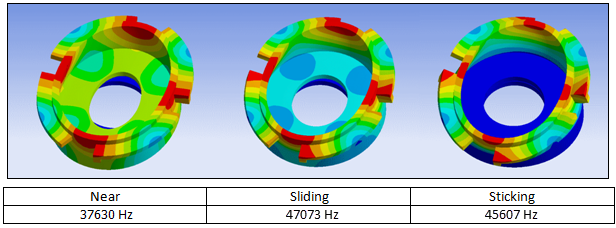
The lowest mode shows nearly independent vibration of the rotor relative to the blade. On the highest mode, sticking reduces this relative movement.
For more information about post-processing for Cyclic Symmetry, and especially on features for postprocessing degenerate Harmonic Indices (those between 0 and N/2), see the Reviewing Results for Cyclic Symmetry in a Modal Analysis section in the Mechanical User's Guide.
Congratulations! You have completed the tutorial.