Chapter 18: Fatigue Analysis of Short Fiber Composite Materials

In this tutorial, you will use the Short Fiber Composite SN Analysis in the DesignLife Add-on to carry out a fatigue analysis on a typical test coupon, which has been manufactured by machining an injection moulded flat plate. This analysis capability has been targeted at short fiber injection-moulded composites, but is in principle also applicable to laminates.

Analysis Type	Fatigue
Features Demonstrated	DesignLife Add-on, DesignLife system, vibration fatigue, inputs and loading conditions
Licenses Required	Ansys Mechanical Enterprise PrepPost and Ansys nCode Enterprise
Help Resources	DesignLife Add-on
Tutorial Files	FatigueShortFiber.zip

This tutorial guides you through the following topics:

18.1. Problem Description

The challenges in estimating damage in composite materials (as compared with metals) derive from the fact that, in general, composite materials are inhomogeneous and anisotropic. Their physical properties may vary throughout a structure and be strongly directional. In order to obtain any useful estimate of damage, it is essential that the inhomogeneity and anisotropy of the material are taken into account both in the structural FE analysis (defining the load-stress transfer function) and in the fatigue analysis (defining the stress-life relationship).

18.2. Access Data Files

Data files for this tutorial can be found here on the Ansys customer site.

The files you need are:

SHORT_FIBER_TIME_DOMAIN.wbpz - this is the model that you will set up by following the steps below. Copy the file to a working folder and complete the worked example using the copy. Make sure that you have write permission to the working folder.
FOT_Fatigue90deg.csv and FOT_Fatigue0deg.csv - these are the orientation tensor files.
Lomov_coupon_R01.mxd - this is the materials database.

18.3. Review FE Results

This example models a tensile specimen test, held at one end and with an enforced displacement of 0.86 mm at the other end to simulate the maximum load.

First, review the results from the finite element analysis:

Start Workbench, and select File > Open.
Browse to the working folder and select SHORT_FIBER_TIME_DOMAIN.wbpz.
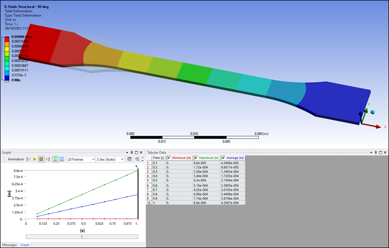
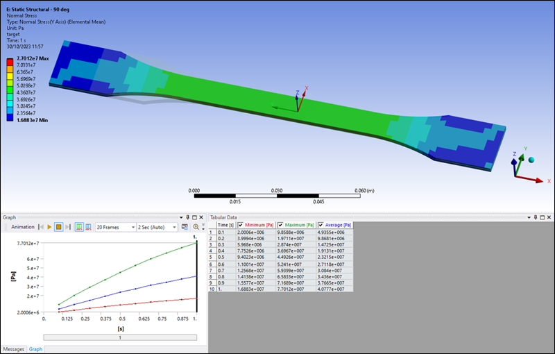
Open the Static Structural - 90 deg system in Mechanical by double-clicking the Model cell and review the different results as shown below:

Total Deformation

Normal Stress

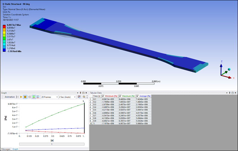
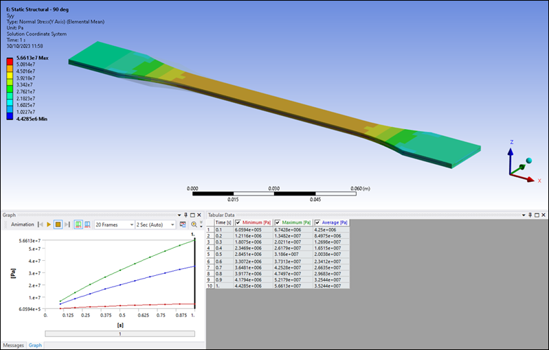
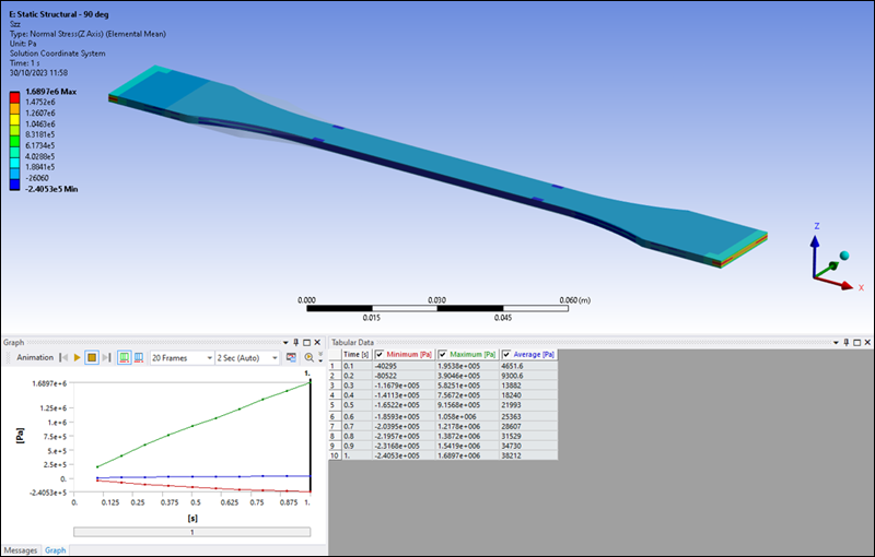
Review the Normal Stress in each direction and note the difference between the different layers:

Normal Stress X-Axis

Normal Stress Y-Axis

Normal Stress Z-Axis

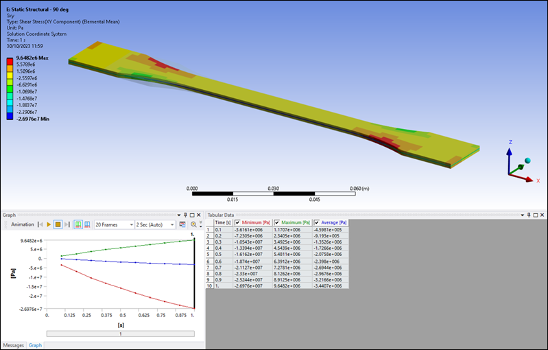
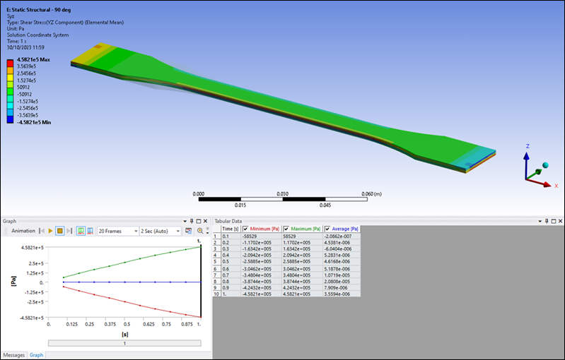
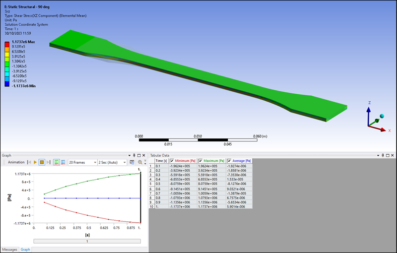
Review the Shear Stress for the different orientations and note the difference between the different layers:

Shear Stress XY Component

Shear Stress YZ Component

Shear Stress XZ Component

18.4. Load the DesignLife Add-on

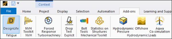
To make the DesignLife capabilities available, click the DesignLife icon in the Add-ons ribbon.
The icon is highlighted in blue, indicating that the add-on is loaded.

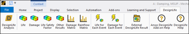
Once the add-on is loaded, the Ansys nCode DesignLife ribbon is visible, exposing all the DesignLife capabilities.

18.5. Insert a DesignLife System

From the DesignLife ribbon, select New Analysis to insert a new DesignLife analysis directly from Mechanical.
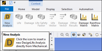
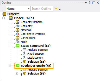
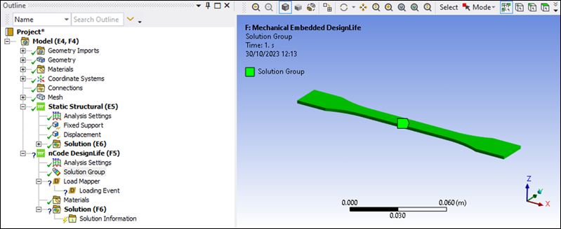
Click the New Analysis icon and verify that the nCode DesignLife (F5) object is inserted into Mechanical.

18.6. Configure Short Fiber Composite Analysis

For this example, you will perform a Short Fiber Composite fatigue calculation using Constant Amplitude loading. The Analysis Domain defaults to the Time based option when the DesignLife system is connected to a Static Structural system.

Select the Short Fiber Composite analysis type to perform the nCode Short Fiber Composite Analysis Engine. This analysis engine performs an SN-based analysis using short fiber, orientation-dependent materials.

The Basquin method is used to define the SN curves for the fatigue calculation (SNMethod) for Short Fiber Composite Analysis. This method uses a set of one or more parameterized stress-life curves and interpolates between them (or extrapolates) based on the share of fibers in the direction of the loading. Each individual SN curve is similar to the standard SN formulation.

The local SN curve will be determined based on a set of SN (Basquin) curves from the nCode MXD database. The corresponding Material Type property for the material map should be set to Short Fiber Composite Basquin Curves. The dataset used for Short Fiber Composite Analysis is the nCodeSFCBasquinCurveContainer.

The only supported Solution Location for Composite Analysis is Element. Results will be recovered from the element centroid. If element centroid results are not available in the FE results file, nCodeDT will average the stresses from the nodes.

The EntityDataType nCode property is set to Stress. Stresses will therefore be recovered from the FE results file. Stresses can result from a static, transient, or modal analysis, but will normally be from an elastic analysis.

Select the Analysis Settings element under nCode DesignLife (F5) and ensure that Analysis Domain is set to Time based.
Set the Analysis Type to Short Fiber Composite. The main objects required for a DesignLife analysis are then generated automatically. These are the Solution Group, Load Mapper and Materials objects.
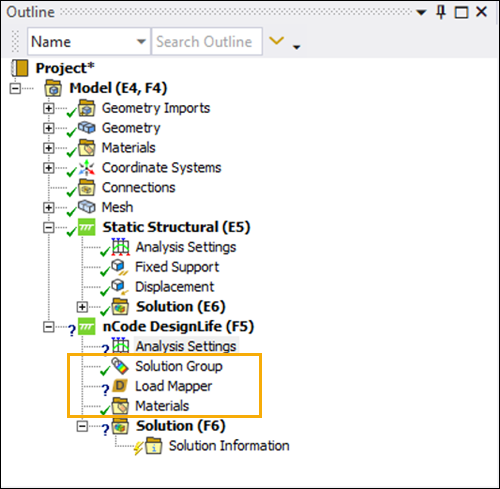
In the Details panel for the Analysis Settings, set the following values:
- Mean Stress Correction to None
- Multiaxial Assessment to Standard
- Combination Method to Abs Max Principal

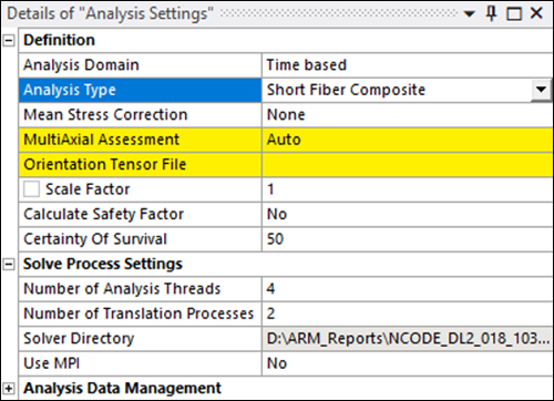
18.7. Define Orientation Tensor File

The Orientation Tensor File must be defined for the Short Fiber Composite analysis. Composites, in general, have anisotropic structures and properties.

The material orientation tensor describes the microstructure in terms of the distribution of fiber orientations at each calculation point (element, layer, section point) in the structure and this information is required if nCodeDT is to take into account the anisotropy of fatigue properties in the analysis.

The material orientation tensor will normally be derived from a simulation of the manufacturing process. The nCode MaterialOrientationTensor property is set to ASCIIFile and the file specified by Orientation Tensor File must be in the Glyphworks-compatible CSV format described under Analysis Settings in the Mechanical Add-ons Guide.

In the Details panel for the Analysis Settings, select FOT_Fatigue90deg.csv from your working folder as the Orientation Tensor File.
Set the Number of Translational Processes to 1.

18.8. Define Inputs and Loading Conditions

The Solution Group defines the portion of the geometry that will be used for the fatigue analysis calculations. By default, all bodies are selected. In the case of this tutorial model, Geometry is therefore set to 2 Bodies.

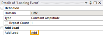
The fatigue loads can be specified as either Constant Amplitude, Time Step or Time Series for the Time based domain.

Select the Load Mapper and click the Add button next to Add Loading Event.
Click Apply. This adds the first Loading Event.
Ensure that the Type for this event is set to Constant Amplitude.
Set the Repeat Count for the Loading Event to 1.
Under Add Load in the Loading Event, click Add and then click Apply.
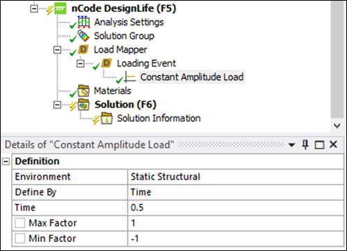
This creates a Constant Amplitude Load object.
Set the following options for the newly-created Constant Amplitude Load object:
- Environment - this selects the system from which the *.rst file will be picked for the nCode fatigue analysis. Select the Static Structural environment so that the results of the static system are used.
- Define By - the loading can be defined by Time or Step. In this case, select Time and then choose the loading corresponding to 0.5 s in the Static Structural system.
- Max Factor - set this parameter to 1.
- Min Factor - set this parameter to -1.
  These two values mean that the FE results will be scaled by 1 (Max Factor) and then by -1 (Min Factor) to form the 2-point constant-amplitude cycle.

18.9. Solve and Review the Results

Right-click the Solution (F6) object in the project tree and select Solve.
While solving, selecting Solution Information will show the solver's progress and display errors as they are encountered.
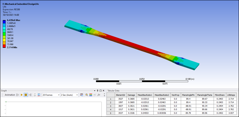
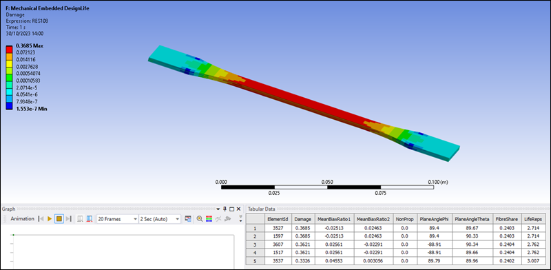
The fatigue results may be viewed as either life or damage. You can add a result by selecting the DesignLife toolbar with the Solution active in the tree.
Alternatively, right-click the Solution (F6) object and insert the following results:
- Select Insert > Life and set the Maximum Life displayed to 1e10.
- Select Insert > Damage and set the Minimum Damage displayed to 1e-10.
Right-click the Solution (F6) object in the project tree and Evaluate all results (see below).

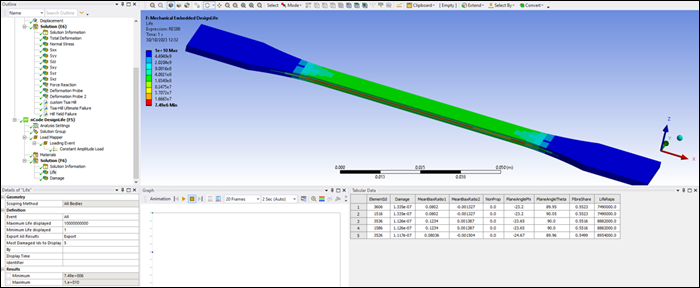
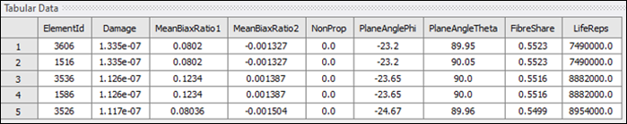
The results are shown as a contour plot in the Mechanical graphics window. The tabular data (below) shows the most damaged ElementID and its corresponding Life or Damage.

18.10. Materials Database Definition

The default materials applied for the analysis are taken from the iceflow_standard.mxd database, which can be found in the mats folder in the nCode installation. When the Analysis Type is set to Short Fiber Composite, the default material is Valox 508 GF30.

You will now modify the default material for Short Fiber Composite analysis:

Scope the body using the Body selection tool in Mechanical.
Select the Materials object under nCode DesignLife (F5) in the project tree.
In the Modify Material Parameters field, click Add.
Click Apply. This creates a new Materials Assignment object.
Click in the Database field and select the Lomov_coupon_R01.mxd as the *.mxd database file where all the nCode materials are defined.
This file is copied to the current directory. The DesignLife Add-on filters the materials found in this database. For Short Fiber Composite, it lists those that are valid for Short Fiber Composite analysis (nCodeSFCBasquinCurveContainer type).
In the Material fields, select the new lomov_coupon material.
Solve again and see how the material assignment impact on the results.

Life Result

Damage Result

You have completed the fatigue analysis and accomplished the overall objective for this tutorial.

Congratulations! You have completed the tutorial.