


In this tutorial, you will perform a fatigue analysis of a simple test specimen with a base excitation acceleration loading using the Mechanical DesignLife Add-on. The loading is described as a Power Spectral Density (PSD), and the fatigue analysis mimics a test sequence employing an electrodynamic shaker.

| Analysis Type | Fatigue |
| Features Demonstrated | DesignLife Add-on, DesignLife system, vibration fatigue, inputs and loading conditions |
| Licenses Required | Ansys Mechanical Enterprise PrepPost and Ansys nCode Enterprise |
| Help Resources | DesignLife Add-on |
| Tutorial Files | FatigueBaseExcitation.zip |
This tutorial guides you through the following topics:
Data files for this tutorial can be found here on the Ansys customer site.
The files you need are:
vib_model_Addon.wbpz - this is the input model that you will set up during the steps defined below. Copy this file to a working folder and complete the worked example using the copy.
vib_model_Addon_completed.wbpz - this is an example of the completed model once all the steps have been followed.
Start Workbench, and select > .
Browse to the working folder and select vib_model_Addon.wbpz.
This Workbench project contains the Harmonic Response system.
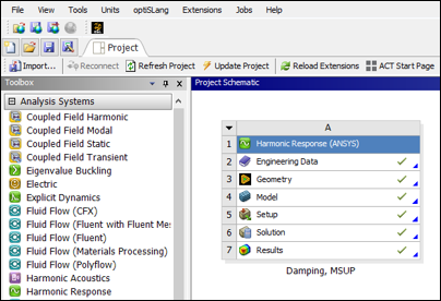
Double click the Results cell to open Mechanical.
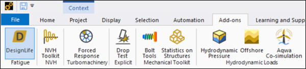
To make the DesignLife capabilities available, click the icon in the ribbon.
The icon is highlighted in blue, indicating that the add-on is loaded.
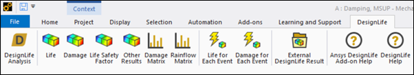
Once the add-on is loaded, the Ansys nCode DesignLife ribbon is visible, exposing all the DesignLife capabilities.
The model consists of a single part, named Surface Body.
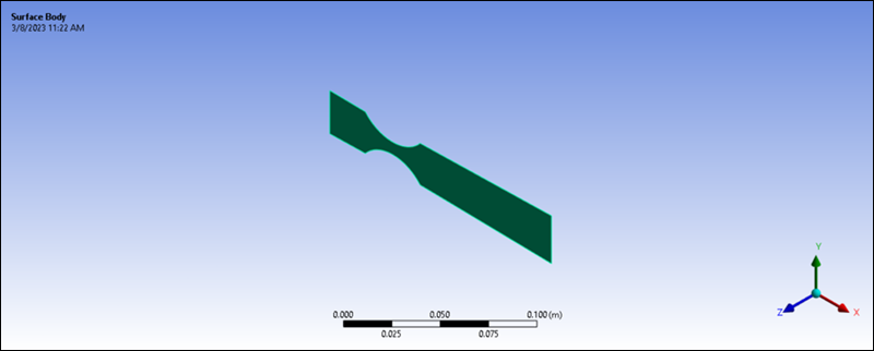
Expand the geometry list, select the Surface Body part, and verify in the Details window for Surface Body that the Material Assignment is
6061-T6.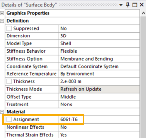
Note:
6061-T6is available as part of the ncode material library. This can be found in the Ansys nCode DesignLife installation under GlyphWorks\mats\nCode_matml.xml.For the fatigue analysis, stress results from a Harmonic Response solution with a unit excitation are needed. The model is of a test specimen, consisting of a plate with a narrowed section. Under test, the specimen is clamped to the test rig at the left end and excited by a 1 g acceleration in the Z-direction. This analysis definition already exists in our project, and the system is already solved.
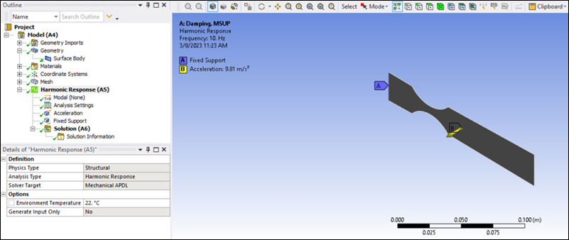
The 1 g acceleration is swept from 10 to 1000 Hz. A constant Damping Ratio of
0.023has been input, and stress results clustered around the model’s natural frequencies have been requested.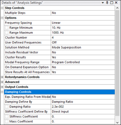
The solution does not need to be updated. The model is already solved and saved with results.
From the DesignLife toolbar, select to insert a new DesignLife analysis directly from Mechanical.
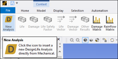
Click the DesignLife Analysis icon and verify that the nCode DesignLife (B5) object is inserted into Mechanical.
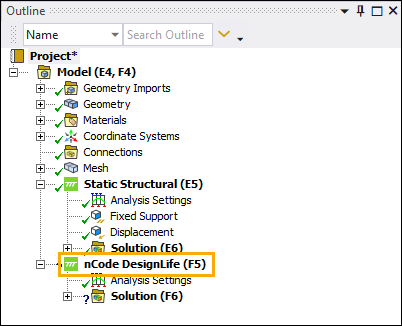
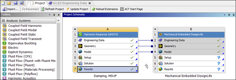
If you return to the Project schematic in Workbench, the system is also visible connected to the Harmonic Response system. The Mechanical Embedded DesignLife system is incorporated into the schematic, sharing Engineering Data, Geometry and Model cells with the Mechanical system.
Setting the DesignLife analysis settings for vibration fatigue.
For this example, you will perform a vibration fatigue calculation using PSD acceleration input. The Analysis Domain defaults to the option when the DesignLife system is connected to a Harmonic system.
Set the Analysis Type to . The main objects required for a DesignLife analysis are then generated automatically. These are the Solution Group, Load Mapper and Materials objects.
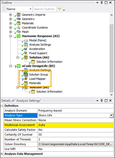
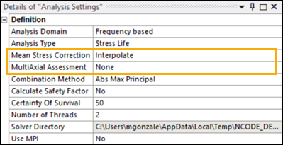
Set the Mean Stress Correction to .
Set the MultiAxial Assessment to .
Leave the rest of Analysis Settings as the default options.
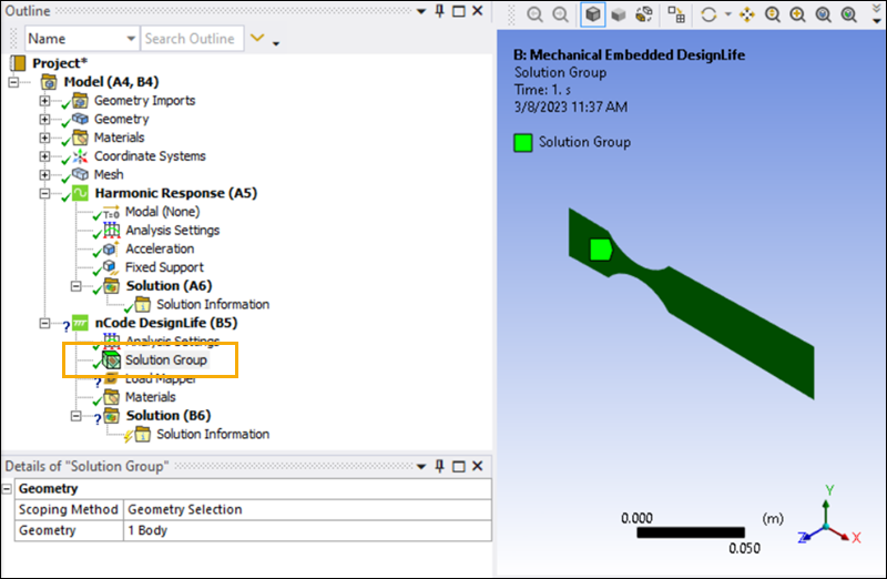
The Solution Group defines the portion of the geometry that will be calculated for the fatigue analysis. By default, all bodies are picked. In this case, there is only one geometry, so there is no need to modify the setting.
The vibration loads can be either PSD, Single Frequency (corresponding to SineDwell), Frequency Range (corresponding to SineSweep), or SineOnRandom in the case of Frequency domain.
The first step is to assign the input as PSD. Select the Load Mapper and click the button within the Add Loading Event. This adds the first loading Event.
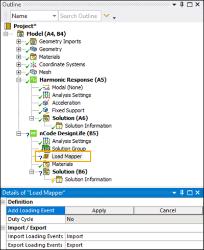
Note: Loading Events in the Analysis Domain can include multiple loadings of the same type. Loading Events in the Analysis Domain can only support one loading case per loading event.
Set the Type to and the Repeat Count to
1, then click the button to add a load under the loading event.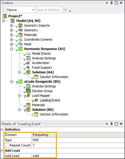
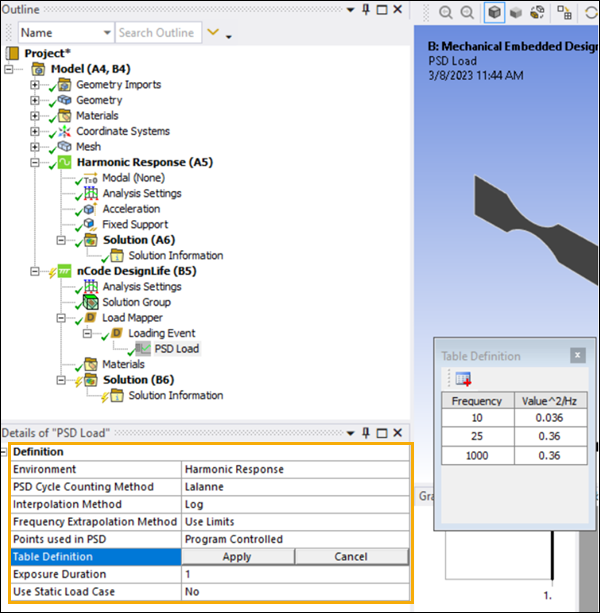
Set the following options for the PSD loading condition:
Environment: This selects the system from which the .rst file will be picked for the nCode fatigue analysis. Select the environment so that the results of the Harmonic Response system are picked.
PSD Cycle Counting Method: This determines the technique used in predicting the probability density function of rainflow ranges from the stress PSD. The available methods are Lalanne, Dirlik, Narrow Band, and Steinberg. The Lalanne and Dirlik methods are the most generally useful, coping with a wide range of loading conditions. The Narrow Band approach, as its name suggests, is suitable only for narrow band conditions; otherwise, it is very conservative. For the current scenario, set the PSD Cycle Counting Method to .
Interpolation Method: This selects the interpolation method for the PSD loading. It can be either linear-linear or log-log. In this case set the Interpolation Method to .
Frequency Extrapolation Method: This sets the frequency extrapolation method for calculating results outside the input frequency ranges. is the default value. If you select to include frequencies outside the range of the input data, the last defined data point will be used.
Points used in PSD: Set this option to , which will use 1024 points by default.
Table Definition: Open the Table Definition and define the following tabular data. Enter the PSD spectrum values into the table and click .
Frequency (Hz) Value2/Hz 100.036250.3610000.36The spectrum values are the frequency versus the loading squared per unit frequency. The Value in the table depends on the loading type. The loading type can be either force, displacement, velocity, or acceleration, but it must match the applied loading from the harmonic analysis. For example, if the applied harmonic loading was 1 g acceleration, then the PSD spectrum values must be defined in g2/Hz.
Exposure Duration: This option is used to determine the length of the excitation, as the input PSD has no timescale associated with it. Set it to
1.Leave Use Static Load Case set to the default value of .
You have defined the input PSD.
Right-click the Solution (B6) object in the project tree and select .
While solving, selecting Solution Information will show the solver's progress and display errors as they are encountered.
The fatigue results may be viewed as either life or damage. You can add a result by selecting the DesignLife toolbar with Solution active in the tree. Alternatively, right-click the Solution (B6) object and insert and results (see below).
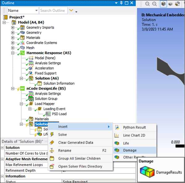
Additional results can be evaluated as follows:
Select > and set the Result to
Select > and set the Result to
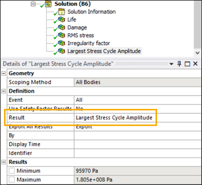
Select > and set the Result to (see below)
Right-click the Solution (B6) object in the project tree and evaluate all the results (see below)
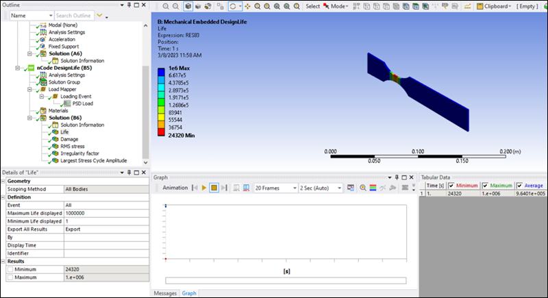
Life Results
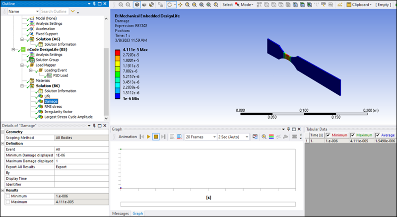
Damage Results
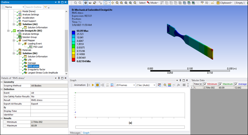
RMS Stress Results
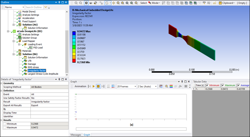
Irregularity Factor Results
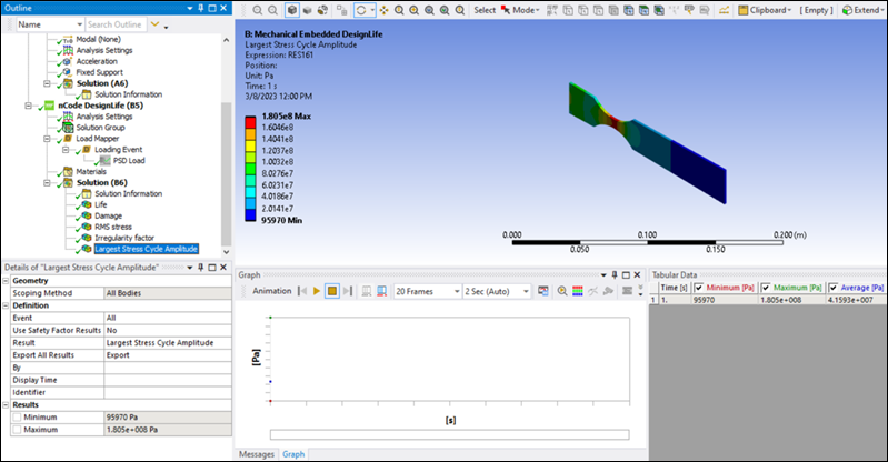
Largest Stress Cycle Amplitude Results
You have completed the fatigue analysis and accomplished the overall objective for this tutorial.
Congratulations! You have completed the tutorial.