


This tutorial demonstrates the capabilities of the Multiharmonic Plot (DPF) result and the Multiharmonic Chart.
| Analysis Type | Multi-harmonic Load Combination |
| Features Demonstrated | Forced Response Add-on, joints, joint loads, springs, coordinate system definition, body view, joint probes |
| Licenses Required | Ansys Mechanical Enterprise/Enterprise Solver/Enterprise PrepPost |
| Help Resources | Forced Response Add-on |
| Tutorial Files | Multiharmonic.zip |
This tutorial guides you through the following topics:
A project has been saved that contains a solved model. The archive contains two systems – a Static Structural (for comparison purposes) and a Harmonic system. Access the file here on the Ansys customer site. The file is titled MH_COMB_001.wbpz.
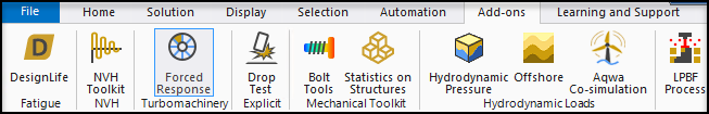
Go to the Add-ons tab and click Forced Response within the ribbon. This will open a new Forced Response tab.
Go to the Harmonic Response System (B5) and review the analysis settings. This is a multi-harmonic analysis.
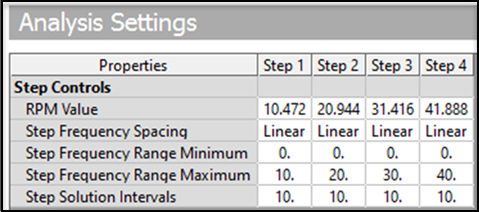
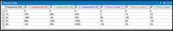
Review the Force and Moment loads under the Harmonic System. They vary with RPM value.
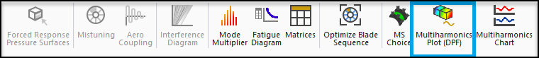
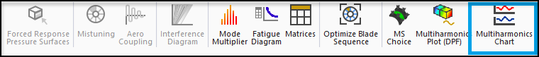
Insert a Multiharmonics Plot (DPF) result object by clicking the Multiharmonic Plot (DPF) object in the Forced Response Add-on ribbon. There is a pre-selected Node in the scoping.
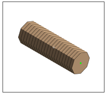
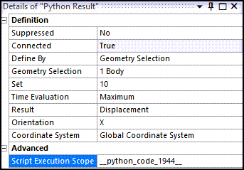
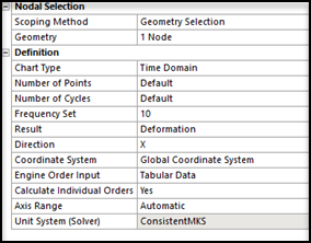
In the Details panel of the Multiharmonic Plot (DPF) result object, click Geometry Selection. Apply the Body Selection filter and click the Beam body to select the Beam object for evaluation. Set the Details panel as shown in the picture below:
Click RMB and choose Evaluate from the context menu.
This will generate a contour plot of the Maximum Displacement result. This displacement result is the combination of all harmonic responses for maximum frequency in all subsets (RPMs).
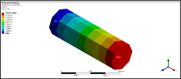
Note: This result matches the UX result from the Static analysis.
Insert a Multiharmonic Chart object by clicking the Multiharmonic Chart object in the Forced Response Add-on ribbon.
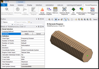
A chart is generated to help determine the contribution of individual orders to the total response seen in Step 6. To achieve this, click Geometry in the Details panel to select scoping. This filters your available scoping types to Nodes or Elements (only these two options are supported). Pick the Node with the highest displacement as seen in Step 6 and set the remaining options as shown in picture below:
Click RMB and select Generate to generate the chart.
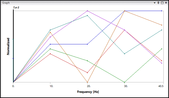
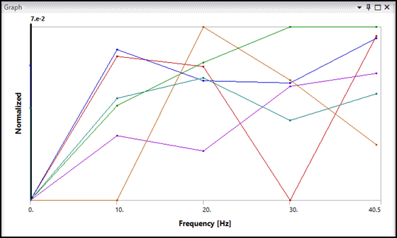
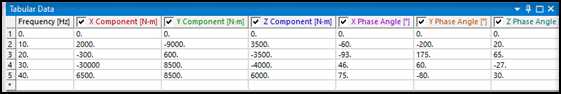
Understanding the Chart: Since the option to Calculate Individual Orders in Frequency domain was chosen, the chart will plot responses for each order and populate the values in a tabular form as seen in the picture below:
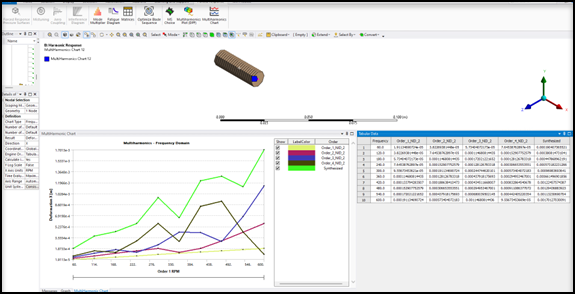
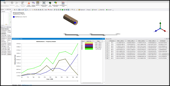
Note: The maximum value shown here for the last frequency is the same as the Maximum obtained in Step 6. To filter out orders 1 and 2, clear the box in the legend.
Plotting the graph in Time Domain: To get the corresponding maximum displacement value in Time Domain, select the same Node and insert another Multiharmonic Chart object. Set the fields as shown in the picture below. The Frequency Set field must be set to 10 to get the values from the last frequencies.
Generate the chart.
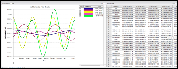
Note: The synthesized Time Domain plot matches the UX plot.
Congratulations! You have completed the tutorial.