This tutorial illustrates how to set up high-pressure gas injection simulations in Ansys Forte. A common application involving such an injection is an internal combustion engine that burns gaseous fuels, such as hydrogen or natural gas. In such applications, the gaseous fuel is injected either into the intake manifold or into the engine cylinder directly. The pressure inside the injector covers a wide range, but it is typically high enough to cause the flow to be supersonic at the injector exit.
The following sections describe the provided files, time required, prerequisites, and a utility for comparing your generated project file (.ftsim) with the one provided in the tutorial download.
This tutorial will cover all the setup steps, but we recommend that you go through the Forte Quick Start Guide first and become familiar with the workflow of the Ansys Forte user interface.
The files for this tutorial are obtained by downloading the
gas_injection.zip file
here .
Unzip gas_injection.zip to your working folder.
Files provided in this tutorial include three Forte project files that has been fully configured as well as a set of facilitating input files that can be used to set up the Forte project starting from a blank project. Specifically, the files include:
hydrogen_injection_tutorial_moving_pintle.ftsim: Fully configured Forte project file that uses the moving pintle (MP) approach.
hydrogen_injection_tutorial_mfr_bc.ftsim: Fully configured Forte project file that uses the mass flow rate boundary condition (MFR-BC) approach.
hydrogen_injection_tutorial_source_model.ftsim: Fully configured Forte project file that uses the source model (SM) approach.
hydrogen_injection_tutorial_with_pintle.tgf: Surface geometry file used by the moving pintle (MP) approach.
hydrogen_injection_tutorial_no_pintle.tgf: Surface geometry file used by the mass flow rate boundary condition (MFR-BC) and source model (SM) approach.
The tutorial sample file is provided as a download. You have the opportunity to select the location for the file when you download and uncompress the sample files.
Note: This tutorial is based on a fully configured sample project that contains the tutorial project settings. The description provided here covers the key points of the project set-up but is not intended to explain every parameter setting in the project. The .ftsim file has all custom and default parameters already configured; the text highlights only the significant points of the tutorial.
The installation includes the cgns_util export command, which you can use to compare the parameter settings in the project file generated at any point during your tutorial set-up against the provided .ftsim, which has the parameter settings for the final, completed tutorial. This command is described in the Forte User's Guide.
Briefly, you can double-check project settings by saving your project and then running the cgns_util to export your tutorial project, and then to export the provided final version of the tutorial. Save both versions and compare them with your favorite diff tool, such as DIFFzilla. If all the parameters are in agreement, you have set up the project successfully. If there are differences, you can go back into the tutorial set-up, re-read the tutorial instructions, and change the setting of interest.
Different hardware configurations impose different requirements for the simulation. For example, if the gas is directly injected into an open space inside the cylinder, it is important to capture the evolution of the morphology of the gas plume accurately because the gas plume shape has large impact on the mixing between the injected gas and the ambient gas (typically air). By contrast, if the gas is injected into a narrow flow passage that causes the gas plume structure to collapse immediately, it will be less critical to capture the detailed transient flow structure of the flow coming through the injector's pintle gap.
In this tutorial, we will describe three different approaches to simulating gas injection and use hydrogen injection as an example. These approaches are illustrated in Figure 12.1: Moving Pintle (MP) approach to modeling gas injection, Figure 12.2: Mass Flow Rate Boundary Condition (MFR-BC) approach to modeling gas injection, and Figure 12.3: Source Model (SM) approach to modeling gas injection. They include:
Moving Pintle (MP): In this approach, the pintle of the injector is modeled as a moving boundary. The fluid domain is split into two regions separated by the pintle seating surfaces: one is the injector region and the other is the main chamber region. The open boundary in the injection region is a pressure boundary. This approach requires the detailed pintle structure be included in the geometry. When the pintle opens or closes, cells in the pintle gap are required to be small, on the order of 30-40 μm. As a result, the time step sizes are relatively smaller than those allowed in the other two approaches. It is the most detailed approach and the most computationally expensive one.
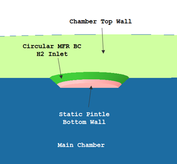
Mass Flow Rate Boundary Condition (MFR-BC): This simplified approach does not involve moving boundary. A ring-shaped surface patch (the circular green surface patch shown in Figure 12.2: Mass Flow Rate Boundary Condition (MFR-BC) approach to modeling gas injection) is carved out on the surface mesh to serve as a mass flow rate inlet. The smallest cells needed can be larger than those required in the moving pintle approach. Mass flow rate, inflow velocity direction and inflow state parameters are specified at the MFR inlet.
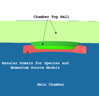
Source Model (SM): In this simplified approach, all the boundaries are defined as static walls. Species (mass) and momentum source models are used to introduce injected hydrogen into the fluid domain. The source domains are the red annulus in Figure 12.3: Source Model (SM) approach to modeling gas injection. Like the mass flow rate boundary condition approach, this approach also allows slightly larger cells and larger time step sizes than those in the moving pintle approach.
These three approaches will be referred to as MP, MFR-BC, SM approaches in this tutorial from now on.
In this tutorial, we will first go through the detailed setup of the MP approach, and then describe the changes needed to set up the MFR-BC and SM approaches. A so-called coupled approach will be used in setting up the two simplified approaches, in which the results sampled in the MP calculation are used as the input of the MFR-BC and SM setup. However, the latter two approaches do not necessarily need to use the coupled approach, for example, instead of using a time-varying mass flow rate profile sampled from the MP calculation, they can use a constant mass flow rate value as their input. At the end of the tutorial, some calculation results will be presented.
In this hydrogen injection example case, hydrogen is injected into a cylindrical chamber filled with nitrogen. The pressure and temperature of the injected hydrogen are 35 bar and 298 K, respectively. The initial pressure and temperature of the nitrogen in the main chamber are 3 bar and 298 K, respectively. The injection starts at time = 0 s and ends at time = 2 ms. The simulation duration is 2.5 ms.
The simulation setup steps follow the top-down order of the setup workflow tree in the Forte Simulate user interface.
Import the surface geometry file
hydrogen_injection_tutorial_with_pintle.tgf using the
Import Geometry ![]() icon on the Geometry panel, select
Surfaces from TGF file as the import method. Keep all the
default import parameters.
icon on the Geometry panel, select
Surfaces from TGF file as the import method. Keep all the
default import parameters.
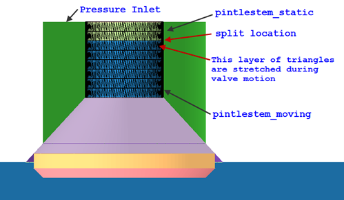
The pintle stem in the imported geometry is a single surface called pintlestem. In this moving pintle configuration, the pintle body will be defined as a moving valve boundary, like the poppet valves in four-stroke internal combustion engines. In Forte, a valve's stem cannot be anchored on an open boundary. Therefore, we need to split pintlestem into two surfaces pintlestem_static and pintlestem_moving. To do the split, right-click surface pintlestem, select Split Mesh and choose the Cut by Plane option. Use X = 0 cm, Y = 0 cm, Z = 0.39 cm as the Point and use X = 0, Y = 0, Z = 1.0 as the Normal for the plane. After the split, rename the two new surfaces as pintlestem_static and pintlestem_moving. The modified surface topology is shown in Figure 12.4: Geometry modification needed for moving pintle boundary. Surface pintlestem_moving and the pintle body below it will be defined as the moving boundary. The top layer of triangles of the pintlestem_moving surface (indicated in Figure 12.4: Geometry modification needed for moving pintle boundary) will be stretched to accommodate the pintle motion.
To facilitate setting up mesh controls and boundary conditions, we create a new reference frame here called RF_Nozzle. Go to Geometry > Reference Frames, click New Reference Frame, name it RF_Nozzle, set New Origin to X = 0 cm, Y = 0 cm, Z = 0.45 cm. In New Orientation, set Rotation about X-axis to 180 degrees and keep the other two axis rotations as zeros.
Note: In this tutorial, it is optional to use such a facilitating reference frame because the location and orientation of the injector are easy to define. However, if the injector's orientation is not aligned with any axis of the global coordinate system, defining a reference frame to anchor the injector can simplify the definition of various mesh controls and boundary motion, in which the word "anchor" means letting the axis of the injector align with one of the coordinate axes of the new reference frame.
Material Point: Set the material point location to X = 0 cm, Y = 0 cm, Z = -2.0 cm.
Global Mesh Size: Set the Global Mesh Size to 0.25 cm.
Three types of refinement controls are used in this project: surface refinement, cone-shaped volume refinement, and solution adaptive meshing (SAM). Detailed refinement control parameters are listed in Table 12.1: Mesh refinement controls used in the MP approach.
Table 12.1: Mesh refinement controls used in the MP approach
| Refinement | Type | Location | Level | Layers |
|---|---|---|---|---|
|
Inlet |
Surface |
inlet |
1/32 |
2 |
|
ChamberTop |
Surface |
chamberwalltop |
1/4 |
2 |
|
Injector |
Surface |
injectorouterwall pintlebottom pintleside pintlestem_moving pintlestem_static pintletop seat |
1/32 |
2 |
|
Cone_4th |
Cone volume |
Ref. Frame for the points: RF_Nozzle Point 1: (0, 0, 0) cm Point 2: (0, 0, 3.0) cm Radius 1: 1.5 cm Radius 2: 2.5 cm |
1/4 |
- |
|
Cone_8th |
Cone volume |
Ref. Frame for the points: RF_Nozzle Point 1: (0, 0, 0) cm Point 2: (0, 0, 3.0) cm Radius 1: 0.5 cm Radius 2: 2.0 cm |
1/8 |
- |
|
Cone_16th |
Cone volume |
Ref. Frame for the points: RF_Nozzle Point 1: (0, 0, 0.25) cm Point 2: (0, 0, 0.8) cm Radius 1: 0.3 cm Radius 2: 0.6 cm |
1/16 |
- |
|
Cone_32th |
Cone volume |
Ref. Frame for the points: RF_Nozzle Point 1: (0, 0, 0.25) cm Point 2: (0, 0, 0.6) cm Radius 1: 0.25 cm Radius 2: 0.45 cm |
1/32 |
- |
|
SAM_H2_MassFrac | SAM Quantity Type = Species Solution Field; Species = h2; Bounds (Absolute Range) = [0.02, 1.0] |
Entire Domain |
1/4 |
- |
|
SAM_VelGrad | SAM Quantity Type = Gradient of Solution Field; Solution Variables = VelocityMagnitude; Bounds = Statistical; Sigma Thresh = 0.25 |
Entire Domain |
1/4 |
- |
Models > Chemistry/Materials: Import a
chemistry set to define the gas phase fluid properties. Click the New
Import Chemistry ![]() icon on the top of the Chemistry/Materials
panel, browse for the /reaction/data/ModelFuelLibrary/Skeletal
folder under your Ansys installation, and open
Hydrogen_MFL2021.cks to load in this chemistry set.
icon on the top of the Chemistry/Materials
panel, browse for the /reaction/data/ModelFuelLibrary/Skeletal
folder under your Ansys installation, and open
Hydrogen_MFL2021.cks to load in this chemistry set.
After the chemistry set has been loaded, you can define two gas mixtures by
clicking the Mixtures ![]() icon in the menu bar. Under gas_mixtures,
click Create New... and then click the edit
icon in the menu bar. Under gas_mixtures,
click Create New... and then click the edit ![]() button to create a new mixture called "Hydrogen", in which you
add h2 as the only species and set its Mass
Fraction to 1.0. Similarly, create another gas mixture called "Nitrogen"
that only includes n2.
button to create a new mixture called "Hydrogen", in which you
add h2 as the only species and set its Mass
Fraction to 1.0. Similarly, create another gas mixture called "Nitrogen"
that only includes n2.
Models > Transport: Since the gas injection involves supersonic flow and it is important to transport total energy instead of transporting internal energy alone, on this panel, turn on the Transport Total Energy option.
This project involves five boundary conditions, one inlet, three static walls, and one moving wall. Detailed setup parameters are listed below:
Inlet: Defined as an inlet boundary
 . Select the gas mixture Hydrogen
as the Composition. Select the
inlet surface as the Location.
Choose Total Pressure as the Inlet
type and set the pressure to 35 bar. The inflow
turbulence conditions are not critical, you can keep the default values or
change the Turbulent Length Scale from the default
1.0 cm to a length smaller than the injector diameter.
Select Total Temperature as the Temperature
Option and set the temperature to 298
K.
. Select the gas mixture Hydrogen
as the Composition. Select the
inlet surface as the Location.
Choose Total Pressure as the Inlet
type and set the pressure to 35 bar. The inflow
turbulence conditions are not critical, you can keep the default values or
change the Turbulent Length Scale from the default
1.0 cm to a length smaller than the injector diameter.
Select Total Temperature as the Temperature
Option and set the temperature to 298
K.ChamberWall: Defined as a wall boundary
 . Select the chamberwallbottom,
chamberwallside, and
chamberwalltop surfaces for
Location. Set Wall Temperature to
298 K. Keep everything else as default on this panel.
. Select the chamberwallbottom,
chamberwallside, and
chamberwalltop surfaces for
Location. Set Wall Temperature to
298 K. Keep everything else as default on this panel.
InjectorWall: Defined as a wall boundary
. Select the injectorouterwall and
seat surfaces for Location. Set
Wall Temperature to 298 K. Keep
everything else as default.PintleStatic: Defined as a wall boundary
. Select the pintlestem_static
surface for Location. Set Wall
Temperature to 298 K. Keep everything else
as default. PintleMoving: Defined as a wall boundary
. This is a moving wall boundary. Select the
pintlebottom, pintleside,
pintlestem_moving, and pintletop
surfaces for Location. Set Wall
Temperature to 298 K. Turn on Wall
Motion and select Offset Table as the
Motion Type. Select Time as
Timing Option. For Lift Profile,
select Create New... and click the
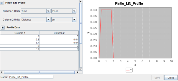
Pencil  icon to create a new lift profile as shown in Figure 12.5: Lift profile of the moving pintle. Note that the units are msec and
cm for the two columns, respectively. Since the tabulated time duration in
the profile is longer than the simulation duration (2.5 ms), it does not
matter whether the Treat Profile As Cyclic option is
checked or not. Set the Direction of the wall motion to
X = 0, Y = 0, Z =
1.0 using RF_Nozzle for Ref.
Frame. Select Valve as the
Movement Type, and multiselect
pintletop and seat as the two
mating surfaces forming the valve gap. Set Valve Motion Activation
Threshold to 0.006 cm and Approx.
Cells in Gap At Min. Lift to 1.5. Using
these valve lift controls, the smallest cells in the valve gap at minimum
lift is required to be smaller than 0.006 cm/1.5 = 0.004 cm = 40 μm.
For global mesh size = 0.25 cm, the refinement level needed is 1/64, which
corresponds to a cell size of 0.25 cm/64 = 0.0039 cm = 39 μm.
icon to create a new lift profile as shown in Figure 12.5: Lift profile of the moving pintle. Note that the units are msec and
cm for the two columns, respectively. Since the tabulated time duration in
the profile is longer than the simulation duration (2.5 ms), it does not
matter whether the Treat Profile As Cyclic option is
checked or not. Set the Direction of the wall motion to
X = 0, Y = 0, Z =
1.0 using RF_Nozzle for Ref.
Frame. Select Valve as the
Movement Type, and multiselect
pintletop and seat as the two
mating surfaces forming the valve gap. Set Valve Motion Activation
Threshold to 0.006 cm and Approx.
Cells in Gap At Min. Lift to 1.5. Using
these valve lift controls, the smallest cells in the valve gap at minimum
lift is required to be smaller than 0.006 cm/1.5 = 0.004 cm = 40 μm.
For global mesh size = 0.25 cm, the refinement level needed is 1/64, which
corresponds to a cell size of 0.25 cm/64 = 0.0039 cm = 39 μm.
This MP configuration requires two regions to be defined, one is the Default Initialization for the main chamber, the other is a material point-based region for the injector.
Default Initialization: Set Initialization Order to 2. Select the gas mixture Nitrogen as the Composition. Set Temperature and Pressure to 298 K and 3.0 bar, respectively. Keep the default for everything else.
Injector_Region: Click the New Secondary Region From Material Point
 icon on the Initial Conditions
panel to create a region called Injector_Region. Set
the material Location to X = 0.18
cm, Y = 0 cm, Z = 0.3
cm. Set Initialization Order to
1. Set Region Type as
Other. Choose the gas mixture
Hydrogen as the Composition. Set
Temperature and Pressure to
298 K and 35.0 bar, respectively.
Keep the default for everything else.
icon on the Initial Conditions
panel to create a region called Injector_Region. Set
the material Location to X = 0.18
cm, Y = 0 cm, Z = 0.3
cm. Set Initialization Order to
1. Set Region Type as
Other. Choose the gas mixture
Hydrogen as the Composition. Set
Temperature and Pressure to
298 K and 35.0 bar, respectively.
Keep the default for everything else.
Simulation Limits: Select Time Based as the Simulation End Point Option and set Max Simulation Time to 2.5 ms.
Time step: Set Initial Simulation Time Step to 1.E-7 s and set constant Max Time Step to 5.E-6 s. The actual time step size will be driven to a value on the order of 1.E-8 s when the pintle is open.
Chemistry Solver: Change the Activate Chemistry option from Always On to Always Off.
Spatially Resolved: Select Time as the Output Timing Control option. Set Interval Based Output Control to output every 0.0001 s. For the Spatially Resolved Species list, select n2 and h2, and turn on the Write Mole Fractions option. For the Solution Variables list, select variables of interest. The minimum variable set should include Pressure, Temperature, Density, Viscosity, VelocityX, VelocityY, VelocityZ, and Velocity Magnitude.
Spatially Averaged: Choose the Time option and set the output interval to 5.0E-7 s. Select n2 and h2 from the species list.
Monitor Probes: On the Monitor Probes setup panel, for the Inquiry Frequency, choose Time as the Time Option and set the interval to 5.0E-7 s.
Important: In this project, we will combine some of the output parameters from the standard CSV output files (such as open_boundary_flow.csv) with the outputs generated by monitor probes. It is important to use the same solution-writing time interval for Spatially Averaged output and Monitor Probes output.
Click the New Probe ![]() icon to add new monitor probes. We will create two
Geometric-based monitor probes to monitor the solution near the injector exit. The
monitored solutions will then be used as the input to set up the simulations of the
MFR-BC and SM approaches.
icon to add new monitor probes. We will create two
Geometric-based monitor probes to monitor the solution near the injector exit. The
monitored solutions will then be used as the input to set up the simulations of the
MFR-BC and SM approaches.
The first probe is called Sphere_R02mm. Select Geometric as the Monitor Type and select Spherical as the Geometric Shape. Set Location to X = 0.32 cm, Y = 0 cm, Z = -0.05 cm in the Global Origin coordinate system and set Radius to 0.02 cm. This monitor probe is mainly used to monitor the flow velocity direction at a location on the X-axis, so the monitored Solution Variables must include VelocityX, VelocityY, VelocityZ, and VelocityMagnitude. Other output parameters are optional.
The second probe is called Annulus. Select Geometric as the Monitor Type and select Annulus as the Geometric Shape. Set the (outer) Radius, Inner Radius, and Annulus Height to 0.34 cm, 0.3 cm, and 0.04 cm, respectively. Define a local coordinate system with origin X = 0.0 cm, Y = 0.0 cm, Z = -0.05 cm in the Global Origin coordinate system to specify the center of the annulus. See the tooltip for the convention used. This monitor probe is mainly used to monitor the following quantities averaged over the annular volume: Temperature, Density, and VelocityMagnitude. Other output parameters are optional.
The Preview Simulation utility is a useful tool for checking
boundary motion, detecting potential surface intersection and verifying volume mesh
generation ahead of the calculation. Open the Mesh Generation
panel under Preview Simulation, select Time
Range as the Time Option, set the
Start, End, and Step
to 0.0 ms, 0.1 ms, and 2.5
ms, respectively. Click the Generate Mesh ![]() icon on the panel to launch Ansys EnSight, and the preview solutions
will be gradually loaded in EnSight as soon as they are created. You can use this
utility to verify the pintle motion.
icon on the panel to launch Ansys EnSight, and the preview solutions
will be gradually loaded in EnSight as soon as they are created. You can use this
utility to verify the pintle motion.
You can choose to run the calculation within the Forte Simulation UI or prepare the run in the UI and then carry out the calculation on a computing cluster. The calculation will generate a set of spatially resolved solutions in .ftind/.ftres format, a standard set of spatially-averaged solution files in .csv format, as well as two .csv files generated by monitor probes, called Sphere_R02mm_probe.csv and Annulus_probe.csv. These files will be used to visualize the solution. Some of them will also be used to set up simulations that use the MFR-BC or SM approach.
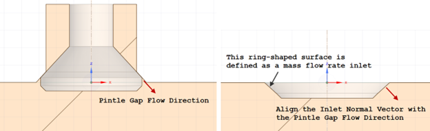
The mass flow rate boundary condition (MFR-BC) approach uses a surface geometry that does not include a moving pintle, so we will set up this case from scratch as a new project.
Import the provided surface geometry file
hydrogen_injection_tutorial_no_pintle.tgf using the
Import Geometry ![]() icon on the Geometry panel, select
Surfaces from TGF file as the import method. Keep all the
default import parameters. In this geometry, a ring-shaped surface called "inlet" is
cut out, and it will be defined as a mass flow rate inlet. Since the inflow velocity
direction of the MFR-BC setup will be obtained from the solution of the MP
calculation, the best practice of defining the normal direction of the inlet surface
is to align the normal vector with the pintle gas flow direction, as shown by the
red arrows in Figure 12.6: Best practice of defining the normal direction of the MFR inlet in geometry
preparation.
icon on the Geometry panel, select
Surfaces from TGF file as the import method. Keep all the
default import parameters. In this geometry, a ring-shaped surface called "inlet" is
cut out, and it will be defined as a mass flow rate inlet. Since the inflow velocity
direction of the MFR-BC setup will be obtained from the solution of the MP
calculation, the best practice of defining the normal direction of the inlet surface
is to align the normal vector with the pintle gas flow direction, as shown by the
red arrows in Figure 12.6: Best practice of defining the normal direction of the MFR inlet in geometry
preparation.
Figure 12.6: Best practice of defining the normal direction of the MFR inlet in geometry preparation
As in the MP setup, we also define a reference frame called RF_Nozzle to facilitate the setup of mesh controls. See the MP setup for the details of this reference frame definition.
The Material Point and Global Mesh Size in this MFR-BC setup are the same as those in the MP setup. See the MP setup for details.
Since this MFR-BC geometry does not include a detailed moving pintle structure, the mesh resolution is allowed to be slightly lower than that in the MP setup in general. Therefore, the deepest refinement level used in this setup is 1/16 (cell size is 0.0156 cm). Adequate mesh resolution is required to resolve the MFR inlet surface slot. There should be at least 3-4 layers of cells across the width of the inlet slot.
The refinement controls used in this MFR-BC setup are listed in Table 12.2: Mesh refinement controls used in the MFR-BC approach.
Table 12.2: Mesh refinement controls used in the MFR-BC approach
| Refinement | Type | Location | Level | Layers |
|---|---|---|---|---|
|
Inlet |
Surface |
inlet |
1/16 |
2 |
|
ChamberTop |
Surface |
chamberwalltop |
1/4 |
2 |
|
Injector |
Surface |
pintlebottom |
1/16 |
2 |
|
Cone_4th |
Cone volume |
Ref. Frame for the points: RF_Nozzle Point 1: (0, 0, 0.43) cm Point 2: (0, 0, 3.0) cm Radius 1: 1.5 cm Radius 2: 2.5 cm |
1/4 |
- |
|
Cone_8th |
Cone volume |
Ref. Frame for the points: RF_Nozzle Point 1: (0, 0, 0.4) cm Point 2: (0, 0, 3.0) cm Radius 1: 0.5 cm Radius 2: 2.0 cm |
1/8 |
- |
|
Cone_16th |
Cone volume |
Ref. Frame for the points: RF_Nozzle Point 1: (0, 0, 0.4) cm Point 2: (0, 0, 0.8) cm Radius 1: 0.4 cm Radius 2: 0.6 cm |
1/16 |
- |
|
SAM_H2_MassFrac | SAM Quantity Type = Species Solution Field; Species = h2; Bounds (Absolute Range) = [0.02, 1.0] |
Entire Domain |
1/4 |
- |
|
SAM_VelGrad | SAM Quantity Type = Gradient of Solution Field; Solution Variables = VelocityMagnitude; Bounds = Statistical; Sigma Thresh = 0.25 |
Entire Domain |
1/4 |
- |
This MFR-BC setup involves three boundary conditions: two static walls and one inlet.
ChamberWall: The Location includes chamberwallbottom, chamberwallside, and chamberwalltop. Set Wall Temperature to 298 K. Keep the default for everything else.
InjectorWall: Set Location to pintlebottom. Set Wall Temperature to 298 K. Keep the default for everything else.
Inlet: Select the gas mixture Hydrogen as the Composition. Select the inlet surface as the Location. If you have a good way to estimate the inflow parameters, you can choose to use constant inputs for mass flow rate, inflow density, etc. In the coupled approach, we use the solutions sampled in the MP calculation to set up the mass flow rate, inflow direction, inflow density and inflow temperature as time-varying profiles. Therefore, we select the Mass Flow Rate, Time Varying option as the Inlet type. The derivation of the time-varying input parameters is described below.
Mass Flow Rate Profile: Create a new time-based MFR profile and name it MFR_Profile. Set column 1 as Time with unit msec and set column 2 as MassFlowRate with unit g/sec. The data can be copied from the open_boundary_flow.csv generated by the MP calculation. The relevant columns in this .csv file are "Time (ms)" and "Mass Flow Rate of Inlet (g/sec)". Since the same units are used in the .csv file and the MFR profile, no unit conversion is needed.
Direction Option: Choose the Axisymmetric Vector, Time Varying option. Set the Origin and Direction of the Axisymmetric Axis to X = 0.0 cm, Y = 0.0 cm, Z = 0.0 cm and X = 0.0, Y = 0.0, Z = 1.0, respectively. Create a new time-based Direction Profile and call it Velocity Direction Profile. Set column 1 as Time with unit msec. Choose Direction, Axisymmetric as the Vector Type. For the axisymmetric vector type, it is assumed that all velocity direction vectors surrounding the specified axisymmetric axis have the same Radial, Tangential, and Axial components. To define these three components, we use the velocities monitored in Sphere_R02mm_probe.csv in the MP calculation to derive the velocity directions. Since this spherical monitor was put on the X-axis, the VelocityX, VelocityY, and VelocityZ monitored can be used to represent the Radial, Tangential, and Axial components. To derive the velocity direction vectors, we simply need to normalize the VelocityX, VelocityY, and VelocityZ by VelocityMagnitude in Sphere_R02mm_probe.csv. This calculation can be done in Excel. Be aware that if the VelocityMagnitude is zero for certain rows, a small tolerance needs to be added to the velocity magnitude to avoid divide-by-zero. Once the normalization calculation is done, use the "Time (ms)" column to fill Column 1 and use the three normalized velocity components to fill Column 2 to 4.
Inflow Mixture Density Option: Choose the Specify Static Density, Time Varying option and create a new time-based Density Profile. We use the densities monitored by the annulus monitor probe in the MP calculation to set up this profile. Set Column 1 as Time with unit msec and set Column 2 as Density with unit g/cm3. Then, simply copy the "Time (ms)" and "Density (g/cm3)" columns of Annulus_probe.csv as column 1 and column 2, respectively, of this density profile.
Temperature Option: Like the density setup, choose the Static Temperature, Time Varying option and create a time-based Temperature Profile. Set Column 1 as Time with unit msec and set Column 2 as Temperature with unit K. Then, simply copy the "Time (ms)" and "Temperature (K)" columns of Annulus_probe.csv from the MP calculation as column 1 and column 2, respectively, of this temperature profile.
This MFR-BC setup only requires the Default Initialization region. Select the gas mixture "Nitrogen" as its Composition and set Temperature and Pressure to 298 K and 3 bar, respectively.
Most of the settings of the source model (SM) approach are the same as those of the MFR-BC approach. The main difference is that the mass and momentum associated with the injected fluid are now introduced into the domain through source models in the SM approach, and all boundary surfaces are now defined as static wall boundaries. In this section, we will only describe the differences in Models and Boundary Conditions with respect to the MFR-BC setup. If you have already set up the MFR-BC case, you can make a copy of the MFR-BC ftsim file and make the modifications described below.
On the Models > Source panel, add a new Species Source and a new Momentum Source.
Species Source:
Select gas mixture Hydrogen as the Species Composition.
For Production Rate, choose the Entire Source Domain, Time Varying as the option, and use the mass flow rate profile MFR_Profile we created for the MFR inlet (in the MFR-BC approach) as the Rate Profile.
Similarly, choose User Specified, Time Varying as the Temperature Option and use the temperature profile created for the MFR inlet (in the MFR-BC approach) as the Temperature Profile.
Use a Bounding Annulus to define the Source Location with the following dimensions:
Point 1: (X = 0.0 cm, Y = 0.0 cm, Z = -0.05 cm), Ref. Frame is Global Origin.
Point 2: (X = 0.0 cm, Y = 0.0 cm, Z = -0.15 cm), Ref. Frame is Global Origin.
Inner Radius 1: 0.35 cm.
Outer Radius 1: 0.45 cm.
Inner Radius 2: 0.35 cm.
Outer Radius 2: 0.45 cm.
Momentum Source:
Select the Entire Source Domain, Time Varying as the Production Rate option. To create the time-based momentum time profile, we will obtain the momentum by multiplying the "Mass Flow Rate of Inlet (g/sec)" column in open_boundary_flow.csv with the "VelocityMagnitude (m/s)" column in Annulus_probe.csv. Both .csv files are outputs from the MP calculation. Note that the velocity unit is m/s in Annulus_probe.csv, so make sure you convert it to cm/s when calculating the momentum if CGS unit will be used as the unit in the momentum profile.
For Momentum Direction, select the Axisymmetric Vector, Time Varying option and use the same configuration (Axis and Direction Profile) as the one used by the MFR inlet (in the MFR-BC approach).
For Source Location, use the same Bounding Annulus as the one used by the Species Source defined above.
You can customize the output parameters on the Output Controls panel based on the output parameters of interest. In Figure 12.7: H2 mole fraction distribution simulated using three different approaches, Figure 12.8: Temperature distribution simulated using three different approaches, and Figure 12.9: Velocity magnitude distribution simulated using three different approaches, simulated H2 mole fraction, temperature, and velocity magnitude contours on a vertical cut-plane using these three different approaches are compared at different times. Although the morphology and penetration lengths are similar among these approaches, there are differences in the detailed flow structure. You can choose a suitable approach depending on the performance or accuracy requirements of each specific project.