This tutorial focuses on the use and implementation of a user-defined function (UDF) and describes how to customize the motion of a component in Ansys Forte. As an example, the 2-stroke engine simulation from Two-Stroke Engine Simulation is here modified to include 3 moving components: the piston, via the built-in crank-slider motion; the crank shaft, via the built-in rotation motion; and the connecting rod, via UDF.
The following sections describe the provided files, time required, prerequisites, and a method for comparing your generated project file (.ftsim) with the one provided in the tutorial download.
This tutorial covers all the set-up steps, but Ansys recommends that you work through the Forte Quick Start Guide first to become familiar with the workflow of the Ansys Forte user interface.
The files for this tutorial are obtained by downloading the
two_stroke_udf.zip file
here .
Unzip two_stroke_udf.zip to your working folder. The
files provided for this tutorial are the following:
2stroke_UDF_tutorial.ftsim:The fully configured Forte project file.
2Stroke_UDF_geometry.tgf: The surface mesh, including all the components.
inletPressureProfile.csv: Data describing the profile of the time-varying pressure for the intake.
All the files related to the UDF are collected inside a UDF_files subfolder:
fsi_UDF_conRod.cpp: The C++ coded UDF.
libForteUDF_conRod.dll: The already compiled, ready-to-use UDF for Windows systems.
libForteUDF_conRod.so: The already compiled, ready to use UDF for Linux systems.
ProjectData.hpp: Supporting UDF file.
HowToCompileTutorial09UDF.txt: The text file containing instructions to recompile or modify the provided UDF.
The tutorial sample file is provided as a download. You have the opportunity to select the location for the file when you download and uncompress the sample files.
Note: This tutorial is based on a fully configured sample project that contains the tutorial project settings. The description provided here covers the key points of the project set-up but is not intended to explain every parameter setting in the project. The .ftsim file has all custom and default parameters already configured; the text highlights only the significant points of the tutorial.
Forte may be launched in a command-line mode to perform certain tasks, such as preparing a run for execution, importing project settings from a text file, or various other tasks described in the Forte User's Guide. One of these tools allows exporting a textual representation of the project data to a text file.
Example
forte.sh CLI -project <project_name>.ftsim -export tutorial_settings.txt
Briefly, you can double-check your tutorial project settings by saving your project and then running the command-line utility to export the settings used in your tutorial project (<project_name>.ftsim), and then use the command a second time to export the settings in the provided final version of the tutorial. Compare them with your favorite diff tool, such as DIFFzilla. If all the parameters are in agreement, you have set up the project successfully. If there are differences, you can go back into the tutorial set-up, re-read the tutorial instructions, and change the setting of interest.
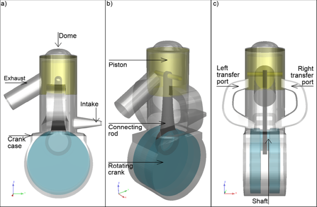
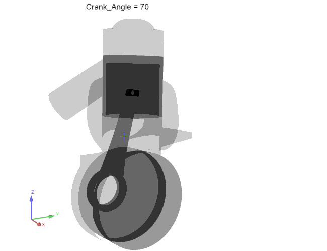
In this case, a full 3-D geometry is used to simulate a 2-stroke engine, including combustion. The fuel in this engine is gasoline and is direct-injected into the combustion chamber from a nozzle placed in the dome. The problem considers a full engine, as shown in Figure 10.1: Full engine geometry. The geometry includes the engine housing, an intake port and exhaust port in part a of the figure, alongside two lateral transfer ports in part (c). The 3 moving components are shown in part (b). The piston, colored gold, slides along the engine liner following a translational slider crank motion, the connecting rod, colored black, is attached to the piston through a pin and to the rotating crank through the shaft, and therefore it has a combined motion. Last, the rotating crank, colored teal, simply rotates around its center with an angular velocity of 3167 RPM. Since all three components are moving, it is important when creating the geometry, to account for some clearance between pairs of surfaces, and to keep the curved surfaces sufficiently smooth to avoid unwanted intersections during the simulation.
Table 10.1: Engine configuration details summarizes the details of this diesel engine configuration.
Table 10.1: Engine configuration details
| Item | Value | Units |
|---|---|---|
| Cycle type | 2-stroke | - |
| Fuel injection system | Direct injection, hollow cone | - |
| Compression ratio | 18.68 | - |
| Bore | 7 | cm |
| Stroke | 7.22 | cm |
| Connecting rod length | 11.95 | cm |
| Fuel | Gasoline | - |
Although the TGF format is used in this tutorial, several other formats are also allowed. See the Geometry Import section in the Forte User's Guide for details. When exporting the TGF file from Ansys SpaceClaim, Ansys recommends selecting the Fine option for the Facet Resolution of the TGF file. The maximum edge length should be 5 mm and Angle resolution should not be larger than 6°.
The project setup workflow follows the top-down order of the Workflow tree in the Ansys Forte Simulate interface. The components that are irrelevant to this tutorial project will not be mentioned in this document, and you can simply skip them and use the default model options.
Note: Changed values on any Editor panel do not take effect until you press the Apply button. Always press the Apply button after modifying a value, before moving to a new panel or the Workflow tree.
In this tutorial, we import an existing geometry into Ansys Forte and set up the automatic
mesh generation using a global mesh size and adapting the mesh where extra resolution is
needed. To import the geometry, go to the Workflow tree and click Geometry. This opens the
Geometry icon bar. Click the Import Geometry ![]() icon. In the resulting dialog, pull down and select Surfaces from TGF file, then select the provided TGF file, 2stroke_UDF_geometry.tgf. In the dialog that opens with TGF file
import options, accept the defaults. In exporting this specific geometry from SpaceClaim, our
default CAD tool, we used the Fine option for the facet resolution,
with a maximum edge length of 5 mm and an angle resolution of
6°. Although the TGF format is used in this tutorial and preferred
because it guarantees that each component is represented by a watertight geometry, several
other formats are also allowed. See the Geometry Import section in the Forte User's Guide for
details. No matter which format is used, in all cases, the volume mesh will be automatically
generated during the simulation. Note that once you have imported the geometry, there are a
number of modifications to the Geometry items that you can apply to the current project,
such as scale, rename, transform, invert normals, or delete geometry elements. Use the
Refit
icon. In the resulting dialog, pull down and select Surfaces from TGF file, then select the provided TGF file, 2stroke_UDF_geometry.tgf. In the dialog that opens with TGF file
import options, accept the defaults. In exporting this specific geometry from SpaceClaim, our
default CAD tool, we used the Fine option for the facet resolution,
with a maximum edge length of 5 mm and an angle resolution of
6°. Although the TGF format is used in this tutorial and preferred
because it guarantees that each component is represented by a watertight geometry, several
other formats are also allowed. See the Geometry Import section in the Forte User's Guide for
details. No matter which format is used, in all cases, the volume mesh will be automatically
generated during the simulation. Note that once you have imported the geometry, there are a
number of modifications to the Geometry items that you can apply to the current project,
such as scale, rename, transform, invert normals, or delete geometry elements. Use the
Refit ![]() button to fit the entire geometry in the graphic window. If the
provided TGF surface mesh is used, once imported, it is important to check and confirm that
the surface mesh normals point away from the fluid domain. To check that, display the
normals by right-clicking the surface in question. In this specific tutorial, the normal
vectors of the triangulated surface mesh of the housing and ports already point towards the
exterior of the fluid domain. However, the normal vectors of the 3 solids and moving
components, the piston, crankshaft and connecting rod, should point inwards (away from the
fluid region). Therefore, select the surfaces associated with these three components,
right-click, apply Invert normals.
button to fit the entire geometry in the graphic window. If the
provided TGF surface mesh is used, once imported, it is important to check and confirm that
the surface mesh normals point away from the fluid domain. To check that, display the
normals by right-clicking the surface in question. In this specific tutorial, the normal
vectors of the triangulated surface mesh of the housing and ports already point towards the
exterior of the fluid domain. However, the normal vectors of the 3 solids and moving
components, the piston, crankshaft and connecting rod, should point inwards (away from the
fluid region). Therefore, select the surfaces associated with these three components,
right-click, apply Invert normals.
The Geometry node also allows setting new reference frames to facilitate the rest of the setup. The new reference frames created are listed in Table 10.2: New Reference Frame in global coordinates.
Table 10.2: New Reference Frame in global coordinates
| Reference Frame |
X [cm] |
Y [cm] |
Z [cm] |
| PistonCoordinateTop | 0 | 0 | 21.4 |
| ExhaustPortRef | 0 | -5 | 14 |
| IntakeRef | 0 | 5 | 7 |
| CrankCase | -2 | 0 | 7 |
| Transfer_R | -6.5 | 0 | 10.5 |
| Transfer_L | 6.5 | 0 | 10.5 |
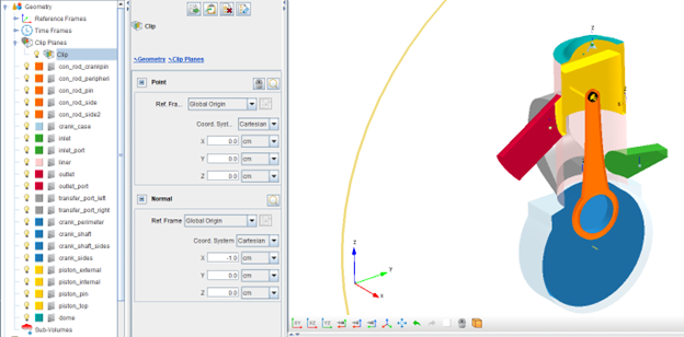
In the already set-up project that you have previously downloaded, you can also see that a clip plane is created to allow a better view of the various components and reference frames, as shown in Figure 10.2: Clip-plane view of the Geometry and Reference Frames.
Automatic mesh generation in Forte requires you to specify a material point, a global mesh size that serves as the reference size for mesh refinement, and various refinement controls. In this tutorial we placed the Material Point 21 cm away from the origin in the positive z-direction, and let the Global Mesh Size be of 4 mm.
Tip: The Material Point being outside of the fluid domain is a commonly encountered setup error, which causes meshing failure. Make sure to set it inside, especially when multiple moving components are involved in the simulation and may change the original volume domain.
Next, we add adaptive and fixed refinement controls, as listed in Table 10.3: Mesh refinement controls.
Table 10.3: Mesh refinement controls
| Item | Ref. type | Ref. location | Ref. level | Ref. layers | Active Range |
| AllSurfaces | Surface |
crank_case, dome, inlet_port, liner, outlet_port | 1/2 | 2 | Always |
| OpenBoundaries | Surface |
inlet, outlet | 1/2 | 2 | Always |
| TDC | Surface |
dome, piston_top | 1/4 | 2 | Always |
| PortWalls | Surface |
inlet_port, outlet_port, transfer_port_left, transfer_port_right | 1/2 | 2 | Always |
| Combustion | Point |
(0, 0, 20.72) cm Radius = 8 cm | 1/2 | - | Always |
| SAM-G |
Solution Adaptive Sol Field = G Lower Bound = -0.3 Upper Bound = 0.3 | Entire Domain | 1/8 | - |
Cyclic Crank Angles From 315° to 415°
|
| SAM-Spray |
Solution Adaptive Grad Sol Field = FuelVaporMassFraction Statistical Sigma = 0.75 | Entire Domain | 1/8 | - | Always |
| Annulusdepth | Annulus |
Point 1: (0, 0, 12) cm Point 2: (0, 0, 21) cm Inner R1 = 3.4 cm Outer R1 = 3.8 cm Inner R2 = 3.4 cm Outer R2 = 3.8 cm | 1/4 | - | Always |
| Crankshaft | Surface | crank_shaft | 1/4 | 2 | Always |
| Spark | Point |
(0, 0, 20.72) cm Radius = 0.4 cm | 1/8 | - |
Cyclic Crank Angles From 315° to 400°
|
| PistonSkirt | Surface | piston_external | 1/4 | 2 | Always |
| Con_rod | Surface |
con_rod_crankpin, con_rod_peripheri, con_rod_pin, con_rod_side, con_rod_side2 | 1/4 | 2 | Always |
In this section the main models parameters are discussed, but you should also refer to the Forte User's Guide for a more complete description of each panel.
Chemistry: Now that the mesh has been set up, assigning models is
next. Assign the chemistry using Models ¬ Chemistry/Materials and use the
New Import Chemistry ![]() icon and select the file
Gasoline_1comp_49sp.cks from the Ansys Forte data
directory. If you are curious, you can view the chemistry details, such as chemistry
source, pre-processing log, gas phase input, gas phase output, thermodynamic input,
transport input, and transport output.
icon and select the file
Gasoline_1comp_49sp.cks from the Ansys Forte data
directory. If you are curious, you can view the chemistry details, such as chemistry
source, pre-processing log, gas phase input, gas phase output, thermodynamic input,
transport input, and transport output.
Flame Speed Model: On the Workflow tree, use Models ¬ Chemistry/Materials ¬ Chemkin Chemistry Set ¬Flame Speed Model and select the Table Library Option. Select Create new..., then add ic8h18 as the fuel species and specify iso_octane as the name. Click Save and close the Library Editor panel. For the Turbulent Flame Speed settings, use a value of 2 for the b1 coefficient and keep the other settings as default. For the Disable Flame Propagation Model option, select the After User-Specified Crank Angle or Time option and set it to 445°. For Unburned Calculation Method, use the Volume Search with Variable Radius option. Click Apply.
This tutorial uses the RANS RNG k-epsilon turbulence model, which is the default turbulence model option. Other turbulence modeling options are available under Models ¬ Transport ¬ Turbulence.
This is a direct-injection case, so turn ON (check) Spray Model in the Workflow tree to display its icon bar (action bar) in the Editor panel. In the panel, keep the defaults. Leave the Use Vaporization Model (default) check ON.
Add an Injector: This Icon bar provides multiple
spray-injector options. For this injector, click the New Hollow Cone
Injector ![]() icon. In the dialog that opens, name the new hollow-cone injector as
Hollow Cone Injector. This opens another icon bar and Editor panel
for the new hollow-cone injector. On the Hollow Cone Injector panel, create a new
Composition, select ic8h18 (iso-octane) in the
Species list, specify the physical properties as
iso-octane, and specify the Mass Fraction as
1.0. Use iso-octane for the Vaporization properties and name the
Composition as gasoline. Click
Save
icon. In the dialog that opens, name the new hollow-cone injector as
Hollow Cone Injector. This opens another icon bar and Editor panel
for the new hollow-cone injector. On the Hollow Cone Injector panel, create a new
Composition, select ic8h18 (iso-octane) in the
Species list, specify the physical properties as
iso-octane, and specify the Mass Fraction as
1.0. Use iso-octane for the Vaporization properties and name the
Composition as gasoline. Click
Save
Now, specify the parameters in Table 10.4: Hollow cone injector settings used in this tutorial
Table 10.4: Hollow cone injector settings used in this tutorial
| Input | Value | Units |
|---|---|---|
| Injected Parcel Count | 30,000 | - |
| Inflow Droplet Temperature | 360 | K |
| Injection Pressure | 50 | bar |
| Inwardly Opening Nozzle | Checked (ON) | - |
| Cone Angle | 54.0 | degrees |
| Liquid Jet Thickness | 15.0 | degrees |
| Droplet Size Distribution | Rosin-Rammler Distribution | - |
| Shape Parameter | 3.5 | - |
| Breakup Length Model Constant | 12.0 | - |
In the Workflow tree under the Hollow Cone Injector node, add a Nozzle. You can either
right-click the Hollow Cone Injector node and select Add or select
that Workflow tree item or use the New Nozzle ![]() icon in the panel's action bar. On the Nozzle Editor panel, set the
parameters as described in Table 10.5: Nozzle settings used in this tutorial. Click
Apply. You can see the nozzle appear at the top of the geometry. (You
may want to make the Geometry non-opaque or change the color of the nozzle itself by
right-clicking in the Workflow tree and selecting Color or
Opacity to make the nozzle easier to see in the interior.)
icon in the panel's action bar. On the Nozzle Editor panel, set the
parameters as described in Table 10.5: Nozzle settings used in this tutorial. Click
Apply. You can see the nozzle appear at the top of the geometry. (You
may want to make the Geometry non-opaque or change the color of the nozzle itself by
right-clicking in the Workflow tree and selecting Color or
Opacity to make the nozzle easier to see in the interior.)
Table 10.5: Nozzle settings used in this tutorial
| Location | |
| Reference Frame | PistonCoordinateTop |
| Coordinate system | Cartesian |
| X | 0.0 cm |
| Y | 0.0 cm |
| Z | -0.05 cm |
| Spray Direction | |
| Reference Frame | PistonCoordinateTop |
| Coordinate System | Spherical |
| Θ | 180 ° |
| Φ | 0.0 ° |
| Nozzle Size | |
| Nozzle Area | 0.001647 cm2 |
After the nozzle is defined, add a new Injection ![]() : On the Injection panel, specify the Start of
Injection as 275 degrees (Cyclic Crank Angle Option), the
Duration of Injection as 12°, specify the
Velocity Profile as a Square Profile, and the
Injected Mass as 7.5 mg.
: On the Injection panel, specify the Start of
Injection as 275 degrees (Cyclic Crank Angle Option), the
Duration of Injection as 12°, specify the
Velocity Profile as a Square Profile, and the
Injected Mass as 7.5 mg.
Spark Ignition: Turn on the spark ignition model by checking the box at Models ¬ Spark Ignition. Keep the defaults for the Spark Ignition settings except Kernel Flame to G-equation Switch Constant = 2.0 and the Flame Development Coefficient = 0.5.
Use the New Spark  icon to create a new spark event and name it
Spark.
icon to create a new spark event and name it
Spark.
Use Models ¬ Spark Ignition ¬ Spark to set up the details of the spark event. In the Location, for Reference Frame, use Global Origin and Cartesian coordinates for the Location, and set X = 0 cm, Y = -1 cm, and Z = 20.3 cm. Select Crank Angle for Timing Option and Starting Angle = 319.0 degrees (Cyclic Crank Angle Option), Duration = 9.0 degrees. Under Spark Energy, set Energy Release Rate = 25.0 J/sec. Accept the default 0.5 for Energy Transfer Efficiency, 0.5 mm (note that the unit is mm) for Initial Kernel Radius, and 3000 for the Number of Flame Particles. Click Apply.
Boundary conditions are set as follows:
Outlet: From the Boundary Conditions node, in the Editor panel,
click the New Outlet  icon and create Outlet. Select the
outlet item in the Location list. Set the
Static Pressure = 0.95 bar and the
Turbulence Boundary Conditions to Turbulent Kinetic Energy
and Length Scale of 3,600 cm2/sec2 and 1.0
cm, respectively.
icon and create Outlet. Select the
outlet item in the Location list. Set the
Static Pressure = 0.95 bar and the
Turbulence Boundary Conditions to Turbulent Kinetic Energy
and Length Scale of 3,600 cm2/sec2 and 1.0
cm, respectively.
Inlet: From the Boundary Conditions node, in the Editor panel,
click the New Inlet  icon and create an Inlet named Inlet. At the top
of the Editor panel, select Create new gas mixture... for the
Composition. Click the Add Species button and then select
o2 (oxygen) and n2 (nitrogen) as the species.
Specify Mass Fraction of 0.23 for
o2 and 0.77 for n2. Name the
composition air and click Save and then
Close. Returning to the Editor panel, select inlet
from the Location list. Select Total Pressure, Time
Varying as the Inlet Option and Crank
Angle as the Time Option. For the pressure profile, select
Create new... and import the pressure profile using the Load
CSV option. The name of the pressure profile is
inletPressureProfile.csv. On the Load CSV dialog, retain the selected
Read Column Titles option. The unit for Column 1 should be
Angle and degrees and for Column 2 the units
should be Pressure and bar. Name the profile
inletPressureProfile and click Save and then
Close. Enable the Repeat Profile Each Cycle
Option. Define Turbulence using values for
Turbulent Kinetic Energy and Length Scale of 3,600
cm2/sec2 and 1.0 cm, respectively. Set the Static
Temperature = 298 K. Click Apply.
icon and create an Inlet named Inlet. At the top
of the Editor panel, select Create new gas mixture... for the
Composition. Click the Add Species button and then select
o2 (oxygen) and n2 (nitrogen) as the species.
Specify Mass Fraction of 0.23 for
o2 and 0.77 for n2. Name the
composition air and click Save and then
Close. Returning to the Editor panel, select inlet
from the Location list. Select Total Pressure, Time
Varying as the Inlet Option and Crank
Angle as the Time Option. For the pressure profile, select
Create new... and import the pressure profile using the Load
CSV option. The name of the pressure profile is
inletPressureProfile.csv. On the Load CSV dialog, retain the selected
Read Column Titles option. The unit for Column 1 should be
Angle and degrees and for Column 2 the units
should be Pressure and bar. Name the profile
inletPressureProfile and click Save and then
Close. Enable the Repeat Profile Each Cycle
Option. Define Turbulence using values for
Turbulent Kinetic Energy and Length Scale of 3,600
cm2/sec2 and 1.0 cm, respectively. Set the Static
Temperature = 298 K. Click Apply.
PistonMoving: This is one of the 3 moving components, and it will
be using the built-in slider crank motion. From the Boundary Conditions node, go to the
Editor panel and click the New Wall  icon and name it PistonMoving. Select the
piston_external, piston_internal and
piston_top items in the Location list. Set the
Thermal Boundary Condition to Wall Temperature,
Constant and 400 K. Turn ON the
Wall Motion option and set the piston Motion Type
to use a Slider Crank with a Stroke of
7.22 cm and a Connecting Rod Length of
11.95 cm with 0.0 Piston Offset. To set the axis
for translation, under Direction, the Reference
Frame is Global Origin and the Coordinate
System is Cartesian. Set X = 0.0 cm,
Y = 0.0 cm, Z = 1.0 cm. Change the
Movement Type to Sliding Interface and select the
liner and piston_external items from the list of
surfaces. For this setting, the moving piston should be selected along with the surface it
is sliding/moving past. Leave the other parameters at their defaults.
icon and name it PistonMoving. Select the
piston_external, piston_internal and
piston_top items in the Location list. Set the
Thermal Boundary Condition to Wall Temperature,
Constant and 400 K. Turn ON the
Wall Motion option and set the piston Motion Type
to use a Slider Crank with a Stroke of
7.22 cm and a Connecting Rod Length of
11.95 cm with 0.0 Piston Offset. To set the axis
for translation, under Direction, the Reference
Frame is Global Origin and the Coordinate
System is Cartesian. Set X = 0.0 cm,
Y = 0.0 cm, Z = 1.0 cm. Change the
Movement Type to Sliding Interface and select the
liner and piston_external items from the list of
surfaces. For this setting, the moving piston should be selected along with the surface it
is sliding/moving past. Leave the other parameters at their defaults.
Pistonpin_conPin: This is moving following the same translation of the PistonMoving boundary condition. The only surface selected in the location list is the piston_pin. The only reason this boundary is treated as a separate one is to impose the Sliding Interface option between another pair of surfaces: con_rod_pin and piston_pin. Other than that, all the parameters are the same as those described for the PistonMoving boundary.
Note: The RPM is specified on the Simulation Controls Editor panel.
Crankshaft: This is the second moving component in this simulation,
and it simply rotates around its center. Click the New Wall icon, select the crank_perimeter,
crank_shaft, crank_shaft_sides, and
crank_sides items in the Location list, and impose
a Wall Temperature of 300 K. Enable Wall
Motion and choose Rotation as the type. Let it rotate at the
origin of the global coordinate system around the
x-direction (Axis Direction of (1.0, 0.0, 0.0)) with an
angular velocity of 3167 RPM. At the bottom of the editor panel, add
the Sliding Interface option, and select the pair of surfaces
con_rod_crankpin and crank_shaft, to avoid any
mesh distortions, any fluid cells in-between, and allow the two surfaces to literally slide
one on top of the other.
ConRod: This is the remaining moving component in this simulation
connected to both the moving piston and the crank shaft surfaces. Due to the combo motion to
which it is subjected (translation in the vertical direction and rotation around the
x-direction), we will use a UDF to describe its motion. Refer to the Simulation Controls
node to see how the UDF is implemented and linked to this project file. Do NOT select any wall motions at this point. The motion will be
imposed only via UDF. For now, treat this boundary as a simple wall. So click the
New Wall icon, select the con_rod_crankpin,
con_rod_peripheri, con_rod_pin,
con_rod_side, con_rod_side2 items in the
Location list, then add a Wall Temperature of
350 K.
IntakePort: Click the New Wall icon and name the new wall IntakePort. Select the
inlet_port item in the Location list and turn
ON the Heat Transfer option and set the
Temperature to 298 K. Now reproduce the
IntakePort with Copy ![]() and Paste
and Paste ![]() , four times, to create four new boundaries as detailed in the following
table.
, four times, to create four new boundaries as detailed in the following
table.
Table 10.6: Details of boundaries created from Copy and Paste operations
| Item | Boundary Name | Location | Wall Temperature |
|---|---|---|---|
| 1 | ExhaustPort | outlet_port | 500 K |
| 2 | Liner | liner | 380 K |
| 3 | Head | dome | 380 K |
| 4 | Crankcase | crank_case | 300 K |
| 5 | TransferPort |
transfer_port_left, transfer_port_right | 298 K |
The domain is initialized with the operating conditions, species concentrations, and temperatures. The Default Initialization species composition is at the expected exhaust composition, assuming complete combustion. The intake and exhaust must also be initialized to the boundary condition values. Set the initialization parameters as described in the following sections.
Default Initialization: Select Default Initialization in the Workflow tree. In the Editor panel, set the Initialization Order to 1. Select Create new gas mixture... for the Composition. This opens the Gas Mixture panel, where you select Add Species. Set a Mass Fraction of o2=0.1123911, n2=0.7421674, co2=0.0996009, and h2o=0.0458404, and Save this composition as exhaust_gas. On the Editor panel, set a Constant Temperature of 1,273 K and a Constant Pressure of 3 bar.
The Turbulence initialization uses the Constant option and the Turbulent Kinetic Energy and Length Scale option with values 3,600 cm2/sec2 and 1.0 cm, respectively. Accept the defaults for the remaining parameters and click Apply.
Now we will create 5 other initialization regions of type Other via
the New Secondary Region From Material Point ![]() option. Follow the instructions in Table 10.7: Initialization region settings.
option. Follow the instructions in Table 10.7: Initialization region settings.
Table 10.7: Initialization region settings
| Region Name | Material Point | Initialization Order | Composition | Temperature | Pressure | Turbulence |
|---|---|---|---|---|---|---|
| Intake |
Ref. Frame IntakeRef (0,0,0) cm | 2 | air | 298 K | 0.755 bar |
TKE = 10,000 cm2/s2 Length scale = 1 cm |
| TransferL |
Ref. Frame Transfer_L (0,0,0) cm | 3 | air | 298 K | 0.755 bar |
TKE = 10,000 cm2/s2 Length scale = 1 cm |
| TransferR |
Ref. Frame Transfer_R (0,0,0) cm | 4 | air | 298 K | 0.755 bar |
TKE = 10,000 cm2/s2 Length scale = 1 cm |
| Exhaust |
Ref. Frame ExhaustPortRef (0,0,0) cm | 5 | exhaust_gas | 773.15 K | 1 bar |
TKE = 10,000 cm2/s2 Length scale = 1 cm |
| BelowPiston |
Ref. Frame CrankCase (0,0,0) cm | 6 | air | 298 K | 0.755 bar |
TKE = 3,600 cm2/s2 Length scale = 1 cm |
On the Simulation Controls node, let the simulation be Crank Angle Based, going from 70° to 430° with 3167 RPM. Select 2-Stroke as the Cycle Type and leave everything else as default.
In the Time Step Editor panel, have the Initial Simulation Time Step as 5e-7 sec, and the Max. Simulation Time Step as 1e-5 sec. Then, in the Advanced Time Step Control Options, double both the Fluid Acceleration Factor and the Rate of Strain Factor from their default values to 1.0 and 1.2 respectively.
In the Chemistry Solver Editor panel, enable the Use Dynamic Cell Clustering to take advantage of groups of cells with similar conditions. Select 2 features to introduce Dynamic Cell Clustering: Max. Temperature Dispersion of 10 K and Max. Equilibrium Ratio Dispersion of 0.05. Then choose to Activate Chemistry > Conditionally > After Fuel Injection Starts and When Temperature is Reached with 600 K as a threshold.
To enable the motion of the connecting rod, the Built-in FSI feature needs to be
turned on. Once enabled, click the New UDF ![]() icon and label it UDF_conrod. In the Editor
panel > UDF Library, browse to the location where you previously
stored the dynamically linked library (*.dll for Windows OS and
*.so for Linux OS) provided with this tutorial. Select the
ConRod boundary condition associated with the connecting rod, and
make sure to have the Global Origin set as the coordinate system used
by the UDF. If you want to recompile or modify the cpp source file, follow the
instructions listed in the HowToCompileTutorial09UDF.txt file
provided with this tutorial.
icon and label it UDF_conrod. In the Editor
panel > UDF Library, browse to the location where you previously
stored the dynamically linked library (*.dll for Windows OS and
*.so for Linux OS) provided with this tutorial. Select the
ConRod boundary condition associated with the connecting rod, and
make sure to have the Global Origin set as the coordinate system used
by the UDF. If you want to recompile or modify the cpp source file, follow the
instructions listed in the HowToCompileTutorial09UDF.txt file
provided with this tutorial.
It is recommended to store the provided dynamic library inside your C:\Program Files\ANSYS Inc\vXXX\reaction\forte.win64\user_defined_functions folder.
Additionally, if you want to include and preview the resulting motion of the customized UDF while performing a Mesh Preview, place a copy of the same *.dll or *.so inside the C:\Program Files\ANSYS Inc\vXXX\reaction\forte.win64\bin folder. It is worth mentioning, that in case you modify this UDF, and the resulting motion depends on any solution fields (for example, pressure), the associated motion will not be shown in the Mesh Preview since at this pre-processing stage no solution field is resolved.
The provided fsi_UDF_conRod.cpp includes multiple commented lines and helper functions that will aid understanding the written code, while providing further examples of general useful operations to modify the UDF itself. Take the time to go through it.
In this section we are focusing on the connecting rod motion implemented in the
fsi_UDF_conRod.cpp file, specifically from lines #496 to #582. The
method: DLL_SO_VOID
Forte_UDF_FSI_Get_Updated_Vertices is called once per boundary per UDF
update cycle. The UDF instance should use this method to provide updated vertex locations
(and optionally velocity) for the specified connecting rod. See Figure 10.3: Sketch of the piston-connecting rod-crank motion.
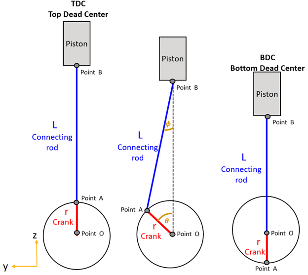
Figure 10.3: Sketch of the piston-connecting rod-crank motion shows a sketch of a piston-crank mechanism in which the piston translates in the z-direction and the crank rotates around the x-direction while being centered at the global origin on point O. The connecting rod moves with a combined motion. Point A, linking the connecting rod with the crank, simply rotates, whereas Point B simply translates. All the other connecting rod points in between A and B have both the translational and the rotational displacement components in the y-z plane.
Inside the DLL_SO_VOID
Forte_UDF_FSI_Get_Updated_Vertices method we find:
Line #499. Every time the UDF updates the connecting rod vertex locations, a message like this is printed out in the MONITOR file
"Entering FSI UDF Vertex Update";
Lines #504 to #515. The slider crank variables (that is, the crank radius and the connecting rod length) are specified.
Lines #518 to #522. The crank angle θ is updated and employed to define the connecting rod angle ϕ as follows:
rsin θ=L sinϕ
Lines #524 to #531. These lines define auxiliary entities needed later in the implementation. They make use of the GLM open-source library that can be downloaded here: https://www.opengl.org/
Lines #533 to #540. Here the connecting rod matrix, M_rod, is built as a sequence of translation, rotation, and again translation operations. Note that the order at which these operations are performed is significant and affects the final result.
Lines #542 to #561. Finally, a for-loop around all the vertex belonging to the connecting rod is performed to update their position, p, via the operation on line #549: p=M_rod*p;
Output controls determine what data are stored for viewing during the simulation and for creating plots, graphs, and animations in Ansys EnSight.
Spatially Resolved: Two different data formats are available: CGNS and DVS. In this tutorial we use CGNS. We set to output spatially resolved data every 20° crank angles and add then a few extra angles around the top dead center location, through the User Defined Crank Angle Outputs option. Variables of interest are selected.
Spatially Averaged and Spray: Opt for Crank Angle in the Spatially Averaged Output Control and set the interval to 1°, then choose the species of interest if any.
Restart Data: It is good practice to enable the restart data writing at the end of a simulation in case you want continue it later. You could also choose to have restart files written at a certain frequency or at specified times depending on your needs.
Monitor Probes: Two spherical probes are set to collect pressure, p, and temperature, T, values over time. The first one is labeled PT_inlet, and averages p and T over a sphere with a 1 mm radius placed inside the intake port, at (0.0, 7.0, 7.2) cm. The second one is named PT_Cylinder_point, and averages p and T over a sphere of 2 mm radius located inside the dome, at (0.0, 0.0, 21.0) cm.
To detect potential problems due to surface intersection and/or
mesh generation before the simulation is started, navigate to the Preview Simulation node. On
the Mesh Generation panel, set the Time Option to
Time for investigating a specific crank angle or to Crank Angle
range for a more extensive investigation, then select Check for Surface
Intersections and/or Include Volume Mesh, depending on what
you are interested in, and finally launch the preview by clicking the Generate
Mesh ![]() icon. Due to the nature of this tutorial, it is appropriate to include
the dynamic library dictating the connecting rod motion inside the Forte
bin folder, as specified in Built-in FSI via UDF. In
this way, code implementation errors and surface intersections can be detected before the
simulation is started, so take advantage of this feature to make sure all the parts behave as
expected and the volume mesh generation are appropriate.
icon. Due to the nature of this tutorial, it is appropriate to include
the dynamic library dictating the connecting rod motion inside the Forte
bin folder, as specified in Built-in FSI via UDF. In
this way, code implementation errors and surface intersections can be detected before the
simulation is started, so take advantage of this feature to make sure all the parts behave as
expected and the volume mesh generation are appropriate.
The run settings depend on the system and environment for your simulations. Change the number of cores used for this simulation according to the resources available to you by navigating to Run Settings ¬ Run Options ¬ Job Script Options ¬ Default MPI Arguments and set the number of cores there. No other changes are needed. You can proceed launching the simulation.
The final section of this tutorial focuses on the results. The animated GIF in Figure 10.4: Full two-stroke motion shows the complete moving path of each component. You can see the piston translating up and down along the z-direction, the crank rotating around the y-axis for an entire revolution, and the connecting rod linking the two via the piston pin and the crank shaft. Note that the reporting crank angle frequency when the piston is approaching the top dead center is slightly increased, giving the eye the impression of a slower RPM. This is just a deliberately imposed post-processing artifact, similar to what you can see in the following figures, to allow a better view of the physics when the spark occurs.
The following Show-Me animation is presented as an animated GIF in Forte's online documentation at the Ansys Help website. If you are reading the PDF version of this manual and want to see the animated GIF, access this section in that online documentation. The interface shown may differ slightly from that in your installed product.
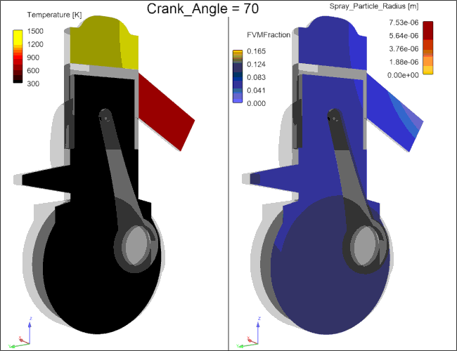
We now cut a y-z plane in the middle of the domain and overlap the temperature contour onto it. We add a 3-D iso-surface based on the G variable, to visualize the advancing flame front (G=0) as it can be seen on the left of Figure 10.5: Temperature distribution and flame front iso-surface on the left and fuel vapor mass fraction distribution and fuel spray parcels on the right. The iso-surface with G=0 is made slightly transparent, and it is colored with the temperature colormap. During the first portion of the cycle the piston is going toward the bottom dead center connecting the exhaust with the main chamber. Then the piston inverts its motion and before approaching the top dead center, at 275° CA, gasoline is injected at 360 K and a darker flow jet can be seen entering from the dome top center. The injected fuel parcels are better visible on the right of Figure 10.5: Temperature distribution and flame front iso-surface on the left and fuel vapor mass fraction distribution and fuel spray parcels on the right. They are colored by their radius size, but for visualization purposes their diameter is kept constant. They lay on a fuel vapor mass fraction contour on the same y-z cut plane as the temperature distribution is shown. At 319° CA the spark takes off and at 323° CA a high temperature kernel is detected on the left side of the figure and expands until the entire combustion chamber is filled.
The following Show-Me animation is presented as an animated GIF in Forte's online documentation at the Ansys Help website. If you are reading the PDF version of this manual and want to see the animated GIF, access this section in that online documentation. The interface shown may differ slightly from that in your installed product.
Figure 10.5: Temperature distribution and flame front iso-surface on the left and fuel vapor mass fraction distribution and fuel spray parcels on the right
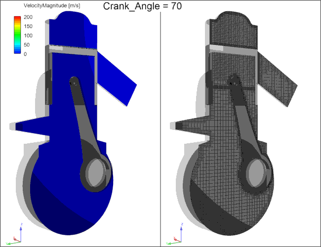
The flow patterns can be better visualized in part a of Figure 10.6: Velocity magnitude contours and vectors on the left and mesh evolution on the right, where the full 2-stroke cycle is reported with the velocity magnitude contour and vectors on the left, while the mesh evolution is displayed on the right of the figure.
The following Show-Me animation is presented as an animated GIF in Forte's online documentation at the Ansys Help website. If you are reading the PDF version of this manual and want to see the animated GIF, access this section in that online documentation. The interface shown may differ slightly from that in your installed product.
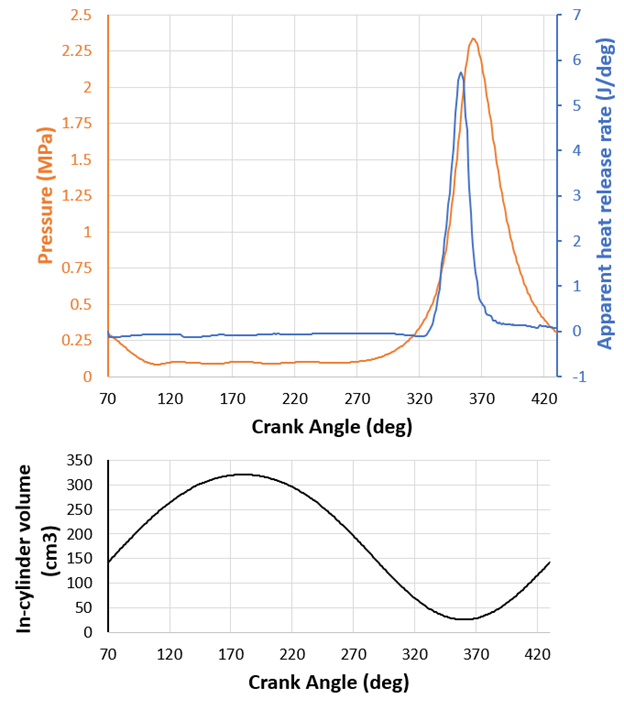
Lastly, in Figure 10.7: In-cylinder spatially averaged pressure, apparent heat release rate and volume, we report the spatially averaged pressure and apparent heat release rate values inside the combustion chamber. A plot of the calculated in-cylinder volume is also reported as part of the usual thermos.csv output file. These results can be further investigated by launching the Forte MONITOR application.