This tutorial describes how to use Ansys Forte to simulate combustion in a direct injection spark ignition internal combustion engine with moving valves. Engine geometry is imported and Ansys Forte's automatic mesh generation is used to create the computational mesh on-the-fly during the simulation.
This section describes the provided files, time required, prerequisites, and a utility for comparing your generated project file (.ftsim) with the one provided in the tutorial download.
We recommend starting with the Ansys Forte Quick Start Guide , which explains the workflow of the Ansys Forte user interface, before doing this tutorial.
The files for this tutorial are obtained by downloading the
siengine_gdi_tutorial.zip file
here
.
Unzip siengine_gdi_tutorial.zip to your working folder.
Forte_GDI_Tutorial.stl: This is the geometry file.
exhaust_valve_lift.csv and intake_valve_lift.csv: Two files of data describing the intake and exhaust valve lifts. Profiles such as these can be imported (from .csv files) or manually entered in the Profile Editor
spatial_output.csv: Specifies when spatially resolved data such as velocity, temperature, species concentrations, etc., will be output.
Forte_GDI_Tutorial.ftsim: A project file of the completed tutorial, for verification or comparison of your progress in the tutorial set-up.
The tutorial sample file is provided as a download. You have the opportunity to select the location for the file when you download and uncompress the sample files.
Note: This tutorial is based on a fully configured sample project that contains the tutorial project settings. The description provided here covers the key points of the project set-up but is not intended to explain every parameter setting in the project. The .ftsim file has all custom and default parameters already configured; the text highlights only the significant points of the tutorial.
Forte may be launched in a command line mode to perform certain tasks such as preparing a run for execution, importing project settings from a text file, or various other tasks described in the Forte User's Guide. One of these tools allows exporting a textual representation of the project data to a text file.
Example
forte.sh CLI -project <project_name>.ftsim -export tutorial_settings.txt
Briefly, you can double-check project settings by saving your project and then running the command-line utility to export the settings in your tutorial project (<project_name>.ftsim), and then use the command a second time to export the settings in the provided final version of the tutorial. Compare them with your favorite diff tool, such as DIFFzilla. If all the parameters are in agreement, you have set up the project successfully. If there are differences, you can go back into the tutorial set-up, re-read the tutorial instructions, and change the setting of interest.
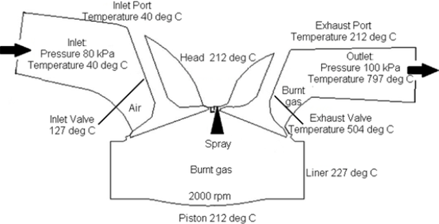
A three-dimensional single cylinder CFD simulation, of a four-stroke spray-guided Gasoline Direct Injection (GDI) Spark Ignition (SI) engine, is performed in this tutorial. Detailed boundary conditions are shown in Figure 7.1: Schematic of GDI engine. Engine simulation is started from intake valve opening (IVO) and fuel is injected during the intake stroke. Homogeneous fuel air mixture is compressed and the spark ignited 15° before compression Top Dead Center (TDC).
This tutorial illustrates the following steps in setting up and solving a Gasoline Direct Injection combustion simulation.
Read an existing geometry into the Forte system.
Define mesh setup and mesh the geometry.
Set up the injection event.
Set up the spark timing event.
Set up the boundary and initial conditions.
Specify the simulation controls.
Specify the output variables and frequency.
Run the simulation.
Examine the results in the report.
The next sections describe how to set up the simulation that is represented in the provided .ftsim file, and some results relating to surfaces, spray, and flame, that you can generate.
Note: All Editor panel options that are not explicitly mentioned in this tutorial should be left at their default values. Changed values on any Editor panel do not take effect until you press the Apply button. Always press the Apply button after modifying a value, before moving to a new panel or to the Workflow tree.
In this tutorial, we will import an existing geometry into Ansys Forte and set up the
automatic mesh generation using a global mesh size and adapting the mesh near the valves.
The geometry used will be half symmetric. To import the geometry, go to the Workflow tree
and click Geometry. This opens the Geometry icon bar. Click the Import
Geometry ![]() icon. In the resulting dialog, pull down and select Surfaces
from one or more STL files. Browse to and select the file called
Forte_GDI_Tutorial. In the dialog that opens with STL file import
options, accept the defaults for units and tolerances. Note that the geometry should always
be in centimeters units when read into Ansys Forte. If it is not, the geometry can be scaled
using the appropriate scaling factor to get it into centimeters. Note that once you have
imported the geometry, there are a number of actions that you can perform on the items in
the Geometry node, such as scale, rename, transform, invert normals, or delete geometry
elements.
icon. In the resulting dialog, pull down and select Surfaces
from one or more STL files. Browse to and select the file called
Forte_GDI_Tutorial. In the dialog that opens with STL file import
options, accept the defaults for units and tolerances. Note that the geometry should always
be in centimeters units when read into Ansys Forte. If it is not, the geometry can be scaled
using the appropriate scaling factor to get it into centimeters. Note that once you have
imported the geometry, there are a number of actions that you can perform on the items in
the Geometry node, such as scale, rename, transform, invert normals, or delete geometry
elements.
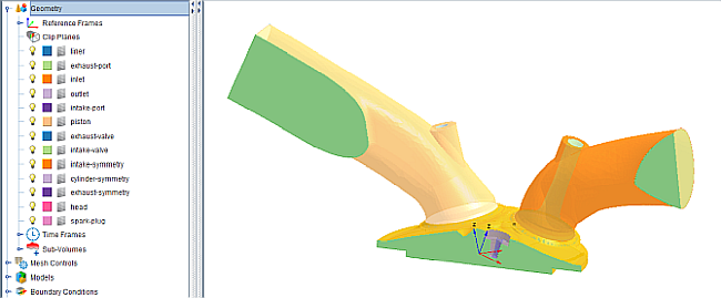
Once the geometry is read in, you should see the following surfaces: liner, exhaust-port, inlet, outlet, intake-port, piston, head, exhaust-valve, intake-valve, intake-symmetry, cylinder-symmetry, exhaust-symmetry, spark-plug.
The Geometry imports in an opaque mode and possibly preset zoom level. It is often
helpful to Refit ![]() the view or use the mouse wheel to re-zoom. To change opacity,
right-click the Geometry node on the left-side Workflow tree and select Medium for the
Opacity level of all geometry elements, as shown in Figure 7.2: Engine geometry with valves and ports defined.
the view or use the mouse wheel to re-zoom. To change opacity,
right-click the Geometry node on the left-side Workflow tree and select Medium for the
Opacity level of all geometry elements, as shown in Figure 7.2: Engine geometry with valves and ports defined.
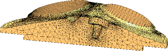
Subvolumes are useful to refine regions of interest, such as the chamber. The subvolume can then be used in the mesh controls to control the size of the mesh in the selected subvolume. Select the following surfaces to define the subvolume: cylinder-symmetry, head, liner, piston, and spark_plug. You should see a triangulated region as in Figure 7.3: Subvolume for the chamber.
The Material Point is the point in the domain that tells Ansys Forte where the mesh will be generated and should be located at least one unit cell length away from any boundaries. This point must remain inside of the domain throughout the entire simulation. Typically it is located near the head so it is still inside the domain at TDC.
Mesh Controls ¬ Material Point: Accept the default Reference Frame using the Global Origin. Set the Location using Cartesian Coord. System to X = 0.25, Y = 3.25, and Z = 0.25 cm. Click Apply.
From the Workflow tree, use Mesh Controls ¬ Global Mesh Size to set the Global Mesh Size to 0.2 cm.
Note: This is the recommended mesh size; a coarser setting of 0.3 cm could be used for tutorial purposes to produce a shorter runtime.
Add a Solution Adaptive Mesh refinement: Click the New Solution Adaptive Mesh
 icon on the Mesh Controls Editor panel, and name the new control
SAM-Temperature. Set the Quantity Type = Gradient of
Solution Field and Solution Variables = Temperature.
Bounds = Statistical and Sigma Threshold =
0.5. Set the Size as Fraction of Global Size = 1/4. The
refinement is Active between Crank Angle 700
and 800 degrees, and the Location option is
Sub-Volumes = chamber. Click Apply.
icon on the Mesh Controls Editor panel, and name the new control
SAM-Temperature. Set the Quantity Type = Gradient of
Solution Field and Solution Variables = Temperature.
Bounds = Statistical and Sigma Threshold =
0.5. Set the Size as Fraction of Global Size = 1/4. The
refinement is Active between Crank Angle 700
and 800 degrees, and the Location option is
Sub-Volumes = chamber. Click Apply.Click the New Solution Adaptive Mesh
icon on the Mesh Controls Editor panel and name the new control
SAM-Velocity. Set the Quantity Type = Gradient of
Solution Field and Solution Variables =
VelocityMagnitude. Bounds = Statistical and
Sigma Threshold = 0.5. Set the Size as Fraction of Global
Size = 1/2. The refinement is Active = Always, and the
Location option is Entire Domain. Click
Apply.Since the G-equation model is used for flame propagation, a SAM control based on the absolute range of G can help keep the flame front zone refined in a more robust way compared to the temperature-gradient–based SAM. Therefore, in addition to temperature-gradient and velocity-gradient–based SAM controls, add a G-value–based SAM. Click the New Solution Adaptive Mesh
icon and name the new control SAM-G. Set the
Quantity Type = Solution Field (DO NOT USE
Gradient of Solution Field) and Solution Variables =
G. Bounds = Absolute
Range, Lower Bound = -0.3 and
Upper Bound = 0.3. Set the Size as
fraction of Global Size = 1/4. The refinement is
Active between Crank Angle 700 and
760 degrees, and the Location option is
Sub-Volumes = chamber. Click Apply. Mesh Controls ¬ Global Mesh Size: Accept the default setting for the Small Feature Deactivation Factor.
Next, you will refine the mesh around key geometric features such as valves and the piston, walls, and open boundaries ("continuative outflows"). The following steps show how the mesh is refined for key geometric features. From the Mesh Controls node, you can add Point, Surface, Line, or Feature Refinements, or Small Feature Avoidance Controls. Create the refinements specified in Table 7.1: Details of the refinement types and settings. These are also good guidelines for the level of refinement for your own engine simulations.
Table 7.1: Details of the refinement types and settings
| Name | Location | Refinement Type | Size Fraction | Cell Layers | Active |
|---|---|---|---|---|---|
| wall | cylinder symmetry, exhaust-symmetry, intake-symmetry, exhaust-port, intake-port, head, piston, liner, spark-plug | Surface | 1/2 | 1 | Always |
| open | inlet, outlet | Surface | 1/2 | 2 | Always |
| spark | 0.551, 0.0945, -0.1678 cm | Point (radius = 0.5 cm) | 1/8 | N/A | Always |
| valves | exhaust-valve, intake-valve | Surface | 1/4 | 2 | Always |
| tdc1 | head, piston, liner | Surface | 1/4 | 2 | 340-380 CA |
| tdc2 | head, piston, liner | Surface | 1/4 | 2 | 700-740 CA |
Chemistry: Now that the mesh has been set up, assigning models is
next. Assign the chemistry with Models ¬ Chemistry/Materials and use the New
Import Chemistry ![]() icon and select the file
Gasoline_1comp_49sp.cks from the Ansys Forte data
directory. If you are curious, you can view the chemistry details, such as chemistry source,
pre-processing log, gas phase input, gas phase output, thermodynamic input, transport input,
and transport output.
icon and select the file
Gasoline_1comp_49sp.cks from the Ansys Forte data
directory. If you are curious, you can view the chemistry details, such as chemistry source,
pre-processing log, gas phase input, gas phase output, thermodynamic input, transport input,
and transport output.
Flame Speed Model: Use Models ¬ Chemistry/Materials ¬ Chemkin Chemistry Set ¬ Flame Speed Model and select the Table Library option in the Laminar Flame Speed drop-down menu. Select Create New..., then add ic8h18 as the fuel species and specify ic8h18_flame_library as the name. For the Turbulent Flame Speed settings, keep the defaults except for Turbulent Flame Speed Ratio (b1), which should be set to 2.0. For Unburned Calculation Method, use the Volume Search with Variable Radius option. Click Apply.
Transport: The default RNG k-epsilon model turbulence settings are used in this tutorial. Those are specified in the Editor panel for Models ¬ Transport ¬ Turbulence. The default fluid properties are also used, which are at Models ¬ Transport.
Spray Model: Turn on the spray model by checking the box at Models ¬ Spray Model. For Spray modeling in Ansys Forte, you will create an Injector first, then and Injection events and Nozzles to the injector. You can have multiple injectors in an Ansys Forte model and they can have different fuels.
Create a new Solid Cone Injector ![]() and name it Solid Injector. Specify the following
for the injector:
and name it Solid Injector. Specify the following
for the injector:
For Composition, select Create New... then add ic8h18 as the fuel species and specify the mass fraction as 1.0. Specify gasoline as the name and click Save.
Set Injection Type to Pulsed Injection and Parcel Specification to Droplet Density with a Droplet Number Density of 1.
Set the Inflow Droplet Temperature to 400K.
For Spray Initialization, select Discharge Coefficient and Angle and specify the Discharge Coefficient as 0.7 and the Cone Angle as 14.0 degrees.
Select Rosin-Rammler Distribution for the Drop Size Distribution, use 3.5 for the Shape Parameter and specify the Initial Sauter Mean Diameter as 120 micron.
Specify the following for the KH and RT model constants:
Size Constant of KH Breakup = 0.5
Time Constant of KH Breakup = 10
Critical Mass Fraction for New Droplet Generation = 0.03
Activate the Impose SMR Conservation in KH Breakup option (Note: This option is typically activated for gasoline injections, but not for diesel injections.)
Size Constant of RT Breakup = 0.1
Time Constant of RT Breakup = 1.0
RT Distance Constant = 1.9
Activate the Use Gas Jet Model and specify 0.5 for the Gas Entrainment Constant.
Now add an Injection by clicking the Injection ![]() icon at the top of the Injector Editor panel or by right-clicking on
the Solid Injector and selecting Add > Injection. Specify the
Injection Type as Pulsed and the
Timing as Crank Angle. Specify the Start
of injection as 420 degrees and the
Duration as 18.4 degrees.
icon at the top of the Injector Editor panel or by right-clicking on
the Solid Injector and selecting Add > Injection. Specify the
Injection Type as Pulsed and the
Timing as Crank Angle. Specify the Start
of injection as 420 degrees and the
Duration as 18.4 degrees.
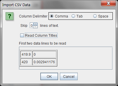
For the Velocity Profile, select Create New..., then click the Load CSV button. Browse to the directory containing the tutorial files and select the file called injection_profile.csv. Clear the Read Column Titles option as shown in Figure 7.4: Import injection profile from CSV dialog.
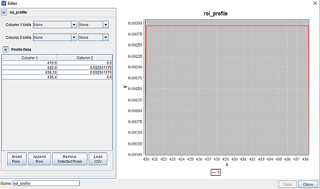
The profile should look like the image in Figure 7.5: Injection profile after import after import. Specify roi_profile as the profile name.
Now that the injection event has been added, we need to specify the nozzles. The nozzles require input for the location, direction, and nozzle hole diameter (or area). Since this is a half-symmetry model, three nozzles will be specified.
On the Solid Injector panel, click the New Nozzle ![]() icon or right-click Solid Injection and click Add >
Nozzle. Name the new nozzle nozzle1.
icon or right-click Solid Injection and click Add >
Nozzle. Name the new nozzle nozzle1.
For the Location, specify X = -5.296 mm, Y = 0.634 mm, and Z = 6.468 mm and for Spray Direction specify X = 3.0415 mm, Y = 2.73735 mm, and Z = -9.12449 mm. For the Nozzle Size, select the Diameter option and specify a nozzle diameter of 300 micron.
Now that the first nozzle has been created, copy and paste nozzle1
and name it nozzle2 using the Copy ![]() and Paste
and Paste ![]() icons. For the Location, specify X =
-5.65 mm, Y = 1.1885 mm, and Z = 6.5991 mm and for
Spray Direction specify X = 1.49781 mm,
Y = 5.08692 mm, and Z = -8.4782 mm.
icons. For the Location, specify X =
-5.65 mm, Y = 1.1885 mm, and Z = 6.5991 mm and for
Spray Direction specify X = 1.49781 mm,
Y = 5.08692 mm, and Z = -8.4782 mm.
Repeat the copy and paste process by copying nozzle2 and naming it nozzle3 to create the last nozzle. For the Location, specify X = -6.7647 mm, Y = 0.72441 mm, and Z = 6.1653 mm and for Spray Direction specify X = -2.90254 mm, Y = 2.74977 mm, and Z = -9.16592 mm.
Now that all the nozzles have been created, they should appear similar to the model in Figure 7.6: Nozzles after specifying location and orientation.

Spark Ignition: Turn on the spark ignition model by checking the box at Models ¬ Spark Ignition.
The spark ignition model defaults include a Min. Kernel Radius for Kernel to G-equation switch of 0.1 cm and Flame Development Coefficient of 1.0. Specify a Kernel Flame to G-equation Switch Constant of 2.0.
Use the New Spark  icon to create a new spark event and name it
Spark.
icon to create a new spark event and name it
Spark.
Use Models ¬ Spark Ignition ¬ Spark to set up the details of the spark event. In the Reference Frame, use Global Origin and Cartesian coordinates for the Location, and set X = 0.551 cm, Y = 0.0945 cm, and Z = -0.1678 cm. Select Crank Angle for Timing Option and Starting Angle = 705 degrees, Duration = 10.0 degrees. Under Spark Energy, set Energy Release Rate = 30.0 J/sec. Accept the default 0.5 for Energy Transfer Efficiency and 0.5 mm (note that the unit is mm) for Initial Kernel Radius. Click Apply.
Boundary conditions are specified for each of the geometry elements in Boundary Conditions ¬ geometry-element-name, where geometry-element-name is each of the items under Geometry in the Workflow tree.
Inlet: From the Boundary Conditions node, click the New
Inlet  icon and create an Inlet. Select inlet from the
Location list. Select Total Pressure as the
Inlet Type with a constant pressure of 8E+04 Pa.
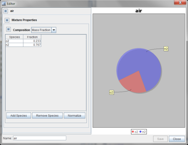
You will set the inlet composition to the correct Mass Fraction values
corresponding to the premixed fuel and air:
icon and create an Inlet. Select inlet from the
Location list. Select Total Pressure as the
Inlet Type with a constant pressure of 8E+04 Pa.
You will set the inlet composition to the correct Mass Fraction values
corresponding to the premixed fuel and air:
o2=0.233
n2=0.767
To do this, select Create new gas mixture... in the
Composition drop-down list above the Location list
and click the Pencil ![]() icon. This opens the Gas Mixture panel, where you select Add
Species and then choose the species you want from the mechanism (see Figure 7.7: Gas Mixture Editor: Defining inlet gas composition). You can find a species more quickly by typing (the beginning
of) the species name to filter the list. Save the inlet gas mixture as
air. You will then see a list to define turbulence using
Turbulent Kinetic Energy and Length Scale of 10000
cm2/sec2 and 1 cm, respectively.
icon. This opens the Gas Mixture panel, where you select Add
Species and then choose the species you want from the mechanism (see Figure 7.7: Gas Mixture Editor: Defining inlet gas composition). You can find a species more quickly by typing (the beginning
of) the species name to filter the list. Save the inlet gas mixture as
air. You will then see a list to define turbulence using
Turbulent Kinetic Energy and Length Scale of 10000
cm2/sec2 and 1 cm, respectively.
Outlet: From the Boundary Conditions node, click the New
Outlet  icon and create Outlet. Select the
outlet geometry item and select the Total Pressure
as the Outlet Type. Give the outlet a Pressure of
1E+05 Pa, which arises from the back-pressure of the exhaust system
with an Offset Distance to Apply Pressure of 0.0
cm. Set the Turbulence Boundary Conditions to
Turbulent Kinetic Energy and Length Scale of 10000
cm2/sec2 and 1 cm, respectively.
icon and create Outlet. Select the
outlet geometry item and select the Total Pressure
as the Outlet Type. Give the outlet a Pressure of
1E+05 Pa, which arises from the back-pressure of the exhaust system
with an Offset Distance to Apply Pressure of 0.0
cm. Set the Turbulence Boundary Conditions to
Turbulent Kinetic Energy and Length Scale of 10000
cm2/sec2 and 1 cm, respectively.
Piston: From the Boundary Conditions node, click the New
Wall  icon and name it Piston. Select the
Piston item in the Location list. Set the
Thermal Boundary Condition to Wall Temperature,
Constant and 485 K. Turn ON the Wall
Motion option and set the piston Motion Type to use a
Slider-Crank Model with a Stroke of 9.0
cm and a Connecting Rod Length of 14.43
cm with 0.0 Piston Offset. Change the Movement
Type to Moving Surface and accept the default
Global Origin Reference Frame. For Direction, the
piston will move along the Z-direction, specify 1.0 for
Z.
icon and name it Piston. Select the
Piston item in the Location list. Set the
Thermal Boundary Condition to Wall Temperature,
Constant and 485 K. Turn ON the Wall
Motion option and set the piston Motion Type to use a
Slider-Crank Model with a Stroke of 9.0
cm and a Connecting Rod Length of 14.43
cm with 0.0 Piston Offset. Change the Movement
Type to Moving Surface and accept the default
Global Origin Reference Frame. For Direction, the
piston will move along the Z-direction, specify 1.0 for
Z.
Intake: Click the New Wall icon and name it intake-port. Select the
intake-port item in the Location list and set the
Temperature to 313 K.
Exhaust: Click the New Wall icon and name it exhaust-port. Select the
exhaust-port item in the Location list and set the
Temperature to 485 K.
Liner: Click the New Wall icon and name it liner. Select the
liner item in the Location list and set the
Temperature to 500 K.
Head: Click the New Wall icon and name it head. Select the
head item in the Location list and set the
Temperature to 485 K.
Intake Valves: Click the New Wall icon and name it intake-valve. The valve
specification is a little more complicated than the stationary walls, such that several
steps are required within the wall panel. These steps specify the wall motion and the way we
want the mesh to adapt to the gap opening near the valve seat when the valve opens or
closes.
Select the intake-valve in the Location list.
Check the Heat Transfer option and set the Temperature to the constant value of 400 K.
Turn ON (check) the Wall Motion and set the Motion Type to Offset Table.
Accept the default Global Origin for the Reference Frame. Select Cartesian for the Coord. System under Direction for the valve motion and set X = 0.241922 cm, Y = 0.0 cm, Z = −0.970296 cm.
To import the lift profile (named intake_valve_lift.csv in the same location as the .stl file you started this tutorial with), select Create new... from the Lift Profile drop-down list and click the Pencil
 icon. In the Profile Editor, click the Load
CSV button and navigate to the
intake_valve_lift.csv file. Clear the
Read Column Titles option and press OK. At the
bottom of the Profile Editor window, name this intake_valve_lift.
Ensure that the units in the first column for Angleare set to
Degrees and the second column for Distance is
set to m. Save the Profile.
icon. In the Profile Editor, click the Load
CSV button and navigate to the
intake_valve_lift.csv file. Clear the
Read Column Titles option and press OK. At the
bottom of the Profile Editor window, name this intake_valve_lift.
Ensure that the units in the first column for Angleare set to
Degrees and the second column for Distance is
set to m. Save the Profile.For Movement Type, change the drop-down menu to Valve. Then select just the surface boundary portion of the valve that comes into contact with the valve seat on the head, as well as the surface boundary that contains the seat region. In this case, select both the head and the intake-valve.
Finally, set the Valve Motion Activation Threshold to 0.02 cm. This indicates that the valve will not open until the lift value specified in the valve-lift profile exceeds this threshold. A smaller value will cause the valves to open sooner, but the mesh refinement required to resolve the gap will be higher. This is a trade-off that will need to be determined based on the goals and outcomes desired from the simulation. In addition to the activation threshold, you may also change the minimum number of cells desired at the smallest gap opening. In this case, specify the Approx. Cells in Gap at Min. Lift as 1.5.
Exhaust Valves: Click the New Wall icon and name it exhaust-valve. Follow a similar
procedure as for the Intake Valves. This time, select the exhaust-valve
item in the Location list and set the Temperature
to 777 K. Turn ON the Wall Motion and set the
Motion Type to Offset Table. Select
Global Origin for the Reference Frame. Select
Cartesian for the Coord. System under
Direction and set X = -0.327218 cm, Y = 0.0 cm,
and Z = -0.944949 cm. Similarly to the intake valves, first import the
.csv (named
exhaust_valve_lift.csv) file, clear the
Read Column Titles option, and name it
exhaust_lift_profile. Then follow the same procedures for specifying
the Movement Type to Valve, selecting the
Valve Seat and Surface it Contacts (exhaust-valve
and head), and setting the Valve Motion Activation
Threshold to 0.02 cm. Specify the Approx. Cells in
Gap at Min. Lift as 1.5.
Symmetry: Click the New Symmetry  icon and name it symmetry. Select the
cylinder-symmetry, exhaust-symmetry, and
intake-symmetry item in the Location list.
icon and name it symmetry. Select the
cylinder-symmetry, exhaust-symmetry, and
intake-symmetry item in the Location list.
Spark Plug: Click the New Wall icon and name it spark-plug. Select the
spark-plug item in the Location list and set the
Temperature to 485 K.
The domain is initialized with the operating conditions, species concentrations and temperatures. The Default Initialization species composition is at the expected exhaust composition, assuming complete combustion. The intake and exhaust must also be initialized to the boundary condition values. Set the following initialization parameters:
Default Initialization:
Select Default Initialization in the Workflow tree. Set the Initialization Order to 2. Since flow goes generally from the intake to the cylinder and then to the exhaust, this indicates that this default (cylinder) region will be the second in the initialization order precedence list.
We will use the Ansys Forte Composition Calculator to compute the exhaust gas composition. Under Utility, select the IVC Calculation
 command in the ribbon or menu. In the Composition calculation,
specify the Fuel Mass (27 mg), select the fuel mixture in the
Liquid input, for Air Flow specify Phi and set
Phi = 1.0, EGR Fraction = 0.0, and for
Internal EGR select the Estimate from CR and
specify a CR of 10. Next, set the
Calculate option to Exhaust and click
Create Mixture. Specify a name of exhaust_gas.
In the Initial Conditions, select exhaust_gas for the
Composition.
command in the ribbon or menu. In the Composition calculation,
specify the Fuel Mass (27 mg), select the fuel mixture in the
Liquid input, for Air Flow specify Phi and set
Phi = 1.0, EGR Fraction = 0.0, and for
Internal EGR select the Estimate from CR and
specify a CR of 10. Next, set the
Calculate option to Exhaust and click
Create Mixture. Specify a name of exhaust_gas.
In the Initial Conditions, select exhaust_gas for the
Composition.Set a Temperature of 1,070 K and the Pressure to 1.05359E+05 Pa.
The Turbulence initialization uses the Turbulent Kinetic Energy and Length Scale option with values 10,000 cm2/sec2 and 1.0 cm, respectively.
The Velocity is initialized using Velocity Components and all the values are set to zero.
Click Apply.
Intake Initialization: The intake manifold Initial Condition is set to match the Boundary Condition at the Inlet. Since this is a separate port that can be closed off from the main cylinder region, we also need to set the equivalent of a material point to identify the region, as well as an initialization order that helps determine what region takes precedence in initializing new cells that appear when gaps are opened.
From the Initial Conditions Workflow tree item, select the New Secondary Region From Material Point
 icon and name it intake.
To identify the region, select a point for the Location under the Reference Frame selection, which is a point that will always be within the Intake port. Set the coordinates for this case to X=-5.6838, Y=1.4295, Z=4.2858 cm, which is a point just inside the inlet.
Set the Initialization Order to 1. Flow is expected to go from the intake to the main region; for this reason, we give it the first order in initialization precedence.
Set the Composition by selecting in the previously saved profile, air. Set the Temperature to 313 K and Pressure to 8.0E+04 Pa. The Turbulence initialization uses Turbulent Kinetic Energy and Length Scale option set to 10,000 cm2/sec2 and 1.0 cm, respectively. Click Apply.
Exhaust Initialization: The Initial Condition of the Exhaust is set to match the Boundary Condition of the Outlet.
From the Initial Conditions Workflow tree item, select the New Secondary Region From Material Point
icon and name it exhaust.To identify the region, select a point for the Location under the Reference Frame selection, which is a point that will always be within the ExhaustPort region. Set the coordinates for this case to X=4.7892, Y=1.5061, Z=3.1552 cm, which is a point just inside the outlet.
Set the Initialization Order to 3. Flow is expected to go from the cylinder to the exhaust port; for this reason, we give it the last order in initialization precedence for the 3 regions defined.
Set the Composition to the existing profile, exhaust_gas. Set the Temperature to 1070K and Pressure to 1.0E+05 Pa.
The Turbulence initialization uses the Turbulent Kinetic Energy and Length Scale option; these are set to 10,000 cm2/sec2 and 1.0 cm, respectively. Click Apply.
Simulation controls allow you to define the simulation limits, RPM, time step, chemistry solver, and transport terms.
Simulation Limits: Use the Simulation Controls panel to select a Crank Angle Based simulation from a CA of 328 to 880.2 degrees. Set RPM = 2,000 rpm. The engine Cycle Type is 4-Stroke.
Time Step: Use Simulation Controls ¬ Time Step and set the following parameters:
Initial Simulation Time Step to 5.0E-7 seconds
Set the Max. Time Step Option to Constant and set the value of Max. Simulation Time Step to 1.E-5 sec. The time step will be adaptively determined throughout the simulation, based on local solution gradients, so this just sets the maximum value allowed. You may also consider reducing the time-step using the Time Varying option. This can be helpful for injection and spark events.
The Advanced Time Step Control Options settings are kept at the defaults:
Time Step Growth Factor = 1.3
Fluid Acceleration Factor = 0.5
Rate of Strain Factor = 0.6
Convection factor = 0.2
Internal Energy Factor = 1.0
Max. Convection Subcycles = 8
Chemistry Solver: Simulation Controls ¬ Chemistry Solver is also kept at the defaults, with the following parameters:
Absolute Tolerance = 1.0E-12
Relative Tolerance = 1.0E-5
Use Dynamic Cell Clustering to take advantage of groups of cells with similar conditions. Select 2 features to introduce Dynamic Cell Clustering: 1) Max. Temperature Dispersion of 10 K and 2) a Max. Equilibrium Ratio Dispersion of 0.05.
To increase the time-to-solution speed, you have the ability to choose when chemistry is activated. In this tutorial, select Conditionally for Activate Chemistry, turn ON (check) After First Spark Event, and select When Temperature is Reached with Threshold Temperature of 600 K. Also select During Crank Angle Interval between 670 and 880 Crank Angle degrees. This ensures that chemistry is active during the time that combustion is expected even if temperature does not rise above 600 K. Click Apply.
Transport Terms: Use the default transport tolerances and maximum number of iterations.
Output controls determine what data are stored for viewing during the simulation and for creating plots, graphs, and animations in Ansys Forte Visualize, CFD-Post, or EnSight.
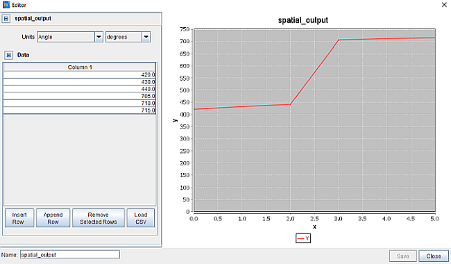
Spatially Resolved: Allows you to control when spatially resolved data such as velocity, temperature, species concentrations, etc., will be output. In the Spatially Resolved panel, set the Interval Based Crank Angle Output to report every 100 degrees (to manage the size of the output file). You can optionally increase the frequency of output during the cycle by selecting User Defined Output Control and importing the spatial_output.csv file, which has a list of specific crank angles where spatially resolved output will occur. Alternatively, you could select User Defined Output Control, and use the Profile Editor to create some other file specifying an output crank-angle profile (the provided profile is illustrated in Figure 7.8: Profile of spatially resolved output control data). Keep the default species and solution variables selected for output. Reducing the variables selected will help reduce file sizes.
Spatially Averaged And Spray: Allows you to control the output of values that are averaged across the domain. On the Spatially Averaged panel, set the Spatially Averaged Output Control to reporting every 1 degree. Keep the default species and solution variables selected for output.
Restart Data: If you anticipate that the case will be stopped and you want the ability to restart it from the last time step solved, select Output Controls ¬ Restart Data. You can specify certain Restart Points using a separate file. Turn on (check) User Defined Restart Points and use the Profile Editor to create a Restart profile. You can view, edit, or import new Restart Points in this 1-D Profile Editor. Sometimes it is helpful in spark ignition cases to save a restart file after IVC but before the spark occurs (CA=687 in this case) so you can use the compression portion of the cycle as a start point in additional runs. Create a new profile for this purpose called restart_output and add two lines with CA value set to 415 and 700 which correspond to points just before injection and spark timing.
You can view the profiles for the Piston, Intake Valves, Exhaust Valves, and Mesh Refinement during the simulation by selecting Preview Simulation > Boundary Motion and clicking the Play icon. This is an excellent way to check whether you have valve overlap and that the settings are correct.
As a method for checking the automatically generated mesh, you can generate a Preview
Mesh. Select Preview Simulation ¬ Mesh Generation. Select Crank
Angle as the Time Option and set it to 720.0
CA. Name the Data Set. Check the Include Volume
Mesh option and then click the Generate Mesh  icon. Next click the Data Set name for viewing in
EnSight. If you want to see the cut plane where the mesh will be generated, create a clip
plane in EnSight. It is a good practice to look at meshes at key points in the cycle such as
Firing Top Dead Center (FTDC), Exhaust Valve Opening (EVO), Intake Valve Closed (IVC), Intake
Valve Open (IVO) and Exhaust Valve Closed (EVC).
icon. Next click the Data Set name for viewing in
EnSight. If you want to see the cut plane where the mesh will be generated, create a clip
plane in EnSight. It is a good practice to look at meshes at key points in the cycle such as
Firing Top Dead Center (FTDC), Exhaust Valve Opening (EVO), Intake Valve Closed (IVC), Intake
Valve Open (IVO) and Exhaust Valve Closed (EVC).
The settings here depend on the system and environment for your simulations. The default for the Run Settings panel is to have nothing selected.
Run Options: Under Job Script Options, change Default Run Type to Parallel and change the default MPI Arguments to 8. (If you do not have MPI installed and configured, keep the default of a serial run).
Windows Settings: This tutorial does not require changes to this panel's defaults; adjust them as necessary for your environment.
Linux Settings: This tutorial does not require changes to this panel's defaults; adjust them as necessary for your environment.
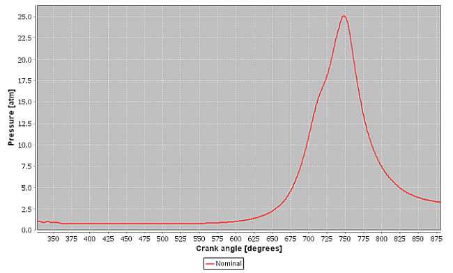
To complete the lesson, select Run Simulation on the Workflow tree and, once Ansys Forte
displays the green START button on the Run Simulation panel and reports a
"Ready" status, click Start. You can monitor the results by clicking on
the Monitor Runs  icon. In the Monitor window that opens, you can select the run you want
to monitor. Open the Ansys Forte Monitor dialog, then select Pressure under
the thermo.csv grouping. The pressure trace should look like the one in
Figure 7.9: Pressure trace result from Forte.
icon. In the Monitor window that opens, you can select the run you want
to monitor. Open the Ansys Forte Monitor dialog, then select Pressure under
the thermo.csv grouping. The pressure trace should look like the one in
Figure 7.9: Pressure trace result from Forte.
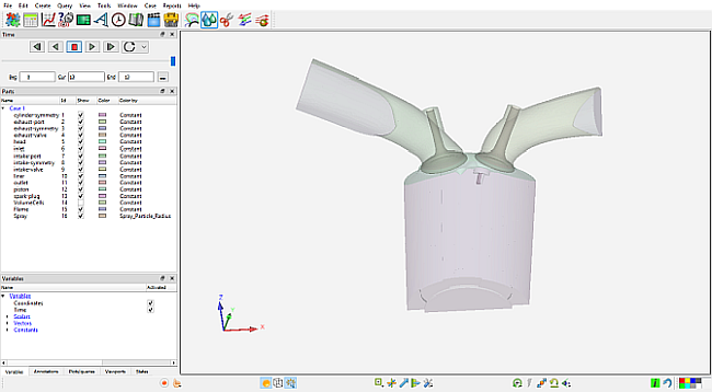
To view the results of the simulation, open the results in Ansys EnSight. In EnSight, open the solution file for the case (Nominal.ftind). Figure 7.10: Screen view of the solution file in EnSight shows the screen view once the solution file has been loaded.
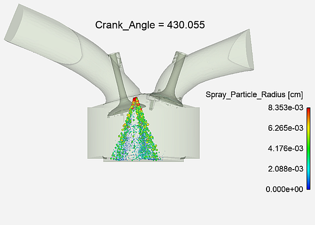
To visualize the spray injection into the chamber, check (turn ON) the Spray in the part list as in Figure 7.11: Turning on the spray particles.
When the spray is activated, all the particles will be a single color. Select and right-click Spray, then Color by > Select variable and then choose Spray Particle Radius as the variable. Right-click the Spray item and click Edit. Check (turn ON) the advanced option at the top right, then click Node, element and line. For Node representation, select Sphere as Type, Scalar as Size by and Spray_Particle_Radius. You can adjust the scale of the spray particles by using the Scale option. In this case, a crank angle of 430.055 is specified. To do this, drag the variable Crank_Angle from the Variable list > Constants > Crank Angle. With these changes, the spray should resemble Figure 7.12: Spray particles in the combustion chamber.
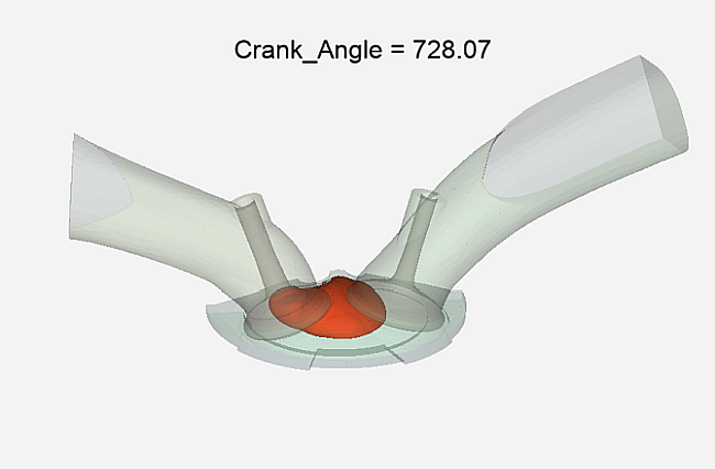
Finally, you may also want to visualize the location of the flame front for spark ignited engines. To visualize the position of the flame, you must create an isosurface. To create an isosurface, select VolumeCells and click Create > Isosurface. Use G as the Variable and set the value to 0.0. Click Create with selected parts. Color the isosurface for a clear view. To see the flame location, the specified crank angle must be after the spark timing, such as at 728CA, as in Figure 7.13: Iso-surface of the flame showing the flame location at 728CA.