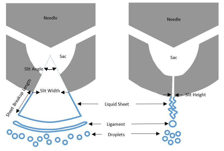
A fan spray is typically injected from a slit injector installed in certain Direct-Injection-Spark-Ignition engines [92] , which is designed to achieve a specific fuel-air mixture preparation requirement. The slit injector uses a planar nozzle with a wide opening angle, allowing spray injected and dispersed into a large space while inducing sufficient air entrainment. The typical inner structure of a slit injector and modeling assumptions are illustrated in Figure 6.7: Modeled processes in a fan spray, front view (left) and side view (right) . It is assumed that a planar liquid sheet is formed when fuel is injected via the nozzle exit. As in hollow-cone sprays, the liquid sheet expands its surface area and thins as it progresses downstream. The shear force exerting on the liquid-air interface causes instability and breaks the sheet into ligaments, where further instability and breakup take place. After the ligaments are broken into droplets, their dynamic and thermodynamic processes are governed by secondary breakup, drag, collision, coalescence, and vaporization.

Figure 6.7: Modeled processes in a fan spray, front view (left) and side view (right)

The liquid sheet formation process is largely determined by the slit geometry and internal nozzle flow conditions. The discharge coefficient is calculated as:

(6–68)

in which is the mass flow rate, is the slit nozzle exit area, calculated as , where is the slit width, is the slit height, and is the slit angle. is the difference between sac pressure and back pressure. It is assumed that the actual area utilized by flow when liquid fuel exits the nozzle can be calculated by . As a result, the injection velocity of the liquid sheet is given by:

(6–69)

The process of the liquid sheet breaking into ligaments is modeled in a similar way as the sheet breakup described in Sheet Breakup . The breakup length is estimated by:

(6–70)

where is the growth rate of the most unstable wave on the surface of the liquid sheet, and the quantity is a tunable constant, taken as 12 by default. Based on mass conservation principles, the liquid sheet thickness at the location of breakup is given by:

(6–71)

And the diameter of the ligament as a result of sheet breakup is calculated as:

(6–72)

where is the wave number corresponding to the maximum growth rate, . As described in Sheet Breakup , in considering the breakup of ligaments into droplets, another linearized instability analysis provides the most unstable wave number on the ligament, denoted as and calculated by Equation 6–65 , which is related to the droplet diameter by Equation 6–64 .

The droplets generated from the liquid sheet and ligament breakup processes will experience secondary breakup, and this is modeled with the TAB model described in Taylor-Analog-Breakup Model . The droplets are also subject to collision and coalescence, aerodynamic drag force, evaporation, and wall impingement; these are the topics of the following sections.