Ansys Forte uses the Arbitrary Lagrangian-Euler (ALE) method [[37] , [70] ] for spatial differencing of the governing equations. For 3-D geometries, this considers a mesh consisting of arbitrary hexahedrons. A control-volume or integral-balance approach [37] is employed, which preserves the local conservation properties of the differential equations. The computational mesh consists of spatial regions, which are composed of cells, the corners of which are the vertices. The vertices are allowed to move in an arbitrarily prescribed manner, enabling piston and valve motion, for example. In addition, when differencing the momentum equations, a different control volume, called a momentum cell, is used. The momentum cells center about the vertices of regular computational cells.
An important advantage of locating the velocities at cell vertices in the ALE method is that this requires no interpolation when determining vertex motion in the Lagrangian stage of the calculation. However, classical ALE method solutions are susceptible to parasitic modes in the velocity field. This problem has been alleviated in FORTÉ by the centering of velocities on cell faces, using the method described by Amsden [3] . Vertex velocities are retained, and momentum associated with the vertices is conserved, but normal velocity components on cell faces are used to compute cell volume changes in Stage 2 and the volume of fluid transported across a cell face in Stage 3. Accelerations of the cell-face velocities due to pressure gradients are calculated by constructing momentum control volumes centered about the cell faces. The volume of any momentum control volume are calculated once the volumes of the main computational cells are determined.
In the finite-difference approximations of Ansys Forte, primary velocities are located at the vertices, such that
 | (5–1) |
Thermodynamic quantities, on the other hand, are primarily located at cell centers:
 | (5–2) |
where Q = p, ρ , T, I, or ρ k , as well as k and ε . Quantities needed at points where they are not primarily located are obtained by averaging neighboring values.
The discretized equations are formed by integrating the differential term in question over the volume of each cell (or momentum cell). Volume integrals of gradient or divergence terms are usually converted into surface area integrals using the divergence theorem. The volume integral of a time derivative is related to the derivative of the integral using Reynolds’ transport theorem [95] . Volume and surface area integrals are performed under the assumption that the integrands are uniform within cells or on cell faces. In this way, area integrals over surfaces of cells are represented as summations over cell faces (or sub-faces):
 | (5–3) |
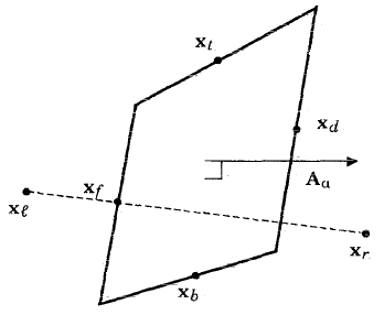
When differencing diffusion terms for a cell-centered quantity Q , it is necessary to evaluate (∇ Q ) α ⋅ A α . Explanation of this calculation requires reference to Figure 5.1: The six points used to define the gradient of cell-centered quantity Q on cell face α . , where the points x l and x r refer to the centers of the cells on either side of face α , and x t , x b , x f and x d are the centers of the four edges bounding face α . We first solve for coefficients a l r , a tb , and a fd such that
 | (5–4) |
Note that since the mesh may be non-orthogonal, the vector x l - x r is not necessarily parallel to A α , and thus a tb and a fd may be nonzero. The finite-difference approximation to (∇ Q ) α ⋅ A α is obtained by applying a dot product with (∇ Q ) α on both sides of both sides of Equation 5–4 with (∇ Q ) α and neglecting terms that are second- and higher-order in the cell dimensions:
 | (5–5) |
In Equation 5–5 Q t is a simple average of the values of Q in the four cells surrounding cell edge " t, " and Q b , Q f , and Q d are defined analogously, relative to edge "b", "f", and "d".
Area integrals over momentum cell faces are ordinarily converted into area
integrals over regular cell faces. This procedure is explained by considering a quantity
Q that is uniform within the regular cells, and then consider the volume
of overlap between a regular cell ( i, j, k ) and the momentum cell
associated with one of its vertices. Three faces of this overlap volume (for example,
a,b,c ) are faces of the momentum cell in question, with outward area vectors
A ’
α , while the other three (for example, d,e,f ) are
surfaces of the regular cell ( i, j, k ), with outward area vectors
¼ A α . The
divergence theorem shows that the integral  over the entire surface of this overlap volume is zero, such that:
 | (5–6) |
In this way, the integral over the three momentum cell faces in question is represented by
 | (5–7) |
and the area vectors A ’ a do not need to be explicitly evaluated. A similar procedure is used to express the outward normal areas A " a of faces of the cell-face control volumes in terms of the regular cell face areas A a .