This tutorial illustrates how to conduct a mesh adaption simulation within Fluent Aero to improve the precision of numerical results. Inside Fluent Aero, you can now enable mesh adaption for all conditions, design points, defined in a simulation. The current mesh adaption inside Fluent Aero uses by default the polyhedral unstructured mesh adaption called PUMA in conjunction with the Combined Hessian Indicator of Fluent. Mesh adaption cycles are used to progressively refine the baseline mesh to reveal the most salient flow features such as shocks, wakes, etc. Inside Fluent Aero, the baseline mesh, the mesh of your imported case or mesh file, will be automatically reloaded between design points. This guarantees that, at each design point, mesh adaption starts from the coarsest mesh of your simulation, the baseline mesh.
In this tutorial, an aircraft, the NASA Common Research Model (CRM) with a wing-body-nacelle pylon (WBNP) configuration, is employed to illustrate this feature. The flight conditions used in this tutorial correspond to the climb and nominal cruise conditions of the Fluent Aero tutorial described in Section 2.3, and are for demonstration purposes only. This tutorial does not require the completion of the above mentioned tutorial.
Note: The main workflow to set-up a mesh adaption simulation in Fluent Aero is described below:
Set up a simulation with one or multiple DPs (conditions).
Enable beta features. In the ribbon go to File->Preferences and inside the Preferences window, select Aero and then enable Beta Features.
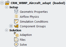
In the Outline View, select Mesh Adaption from Setup. Its UI, named as Adaption, will be automatically displayed under Solution.
Go to Solution → Adaption UI and set up adaption settings.
Go to Solution→Files → Solution Files to set up writing intermediate solution if needed.
Go to Solution→Solve →Iteration to set the total number of iterations for each DP.
Set the DP/DPs status to Needs Update.
Click Solution → Solve →Update to launch the airflow simulation with mesh adaption.
Current limitations of mesh adaption beta feature inside Fluent Aero:
Restart capabilities are not supported.
Saving/reloading mesh adaption settings of each design point is not supported.
Loading and post-processing adapted solutions of each mesh adaption cycle are not supported.
As the adapted mesh size increases with mesh adaption cycles, the computational resource requirements increase. In order to conduct this tutorial, it is recommended to have at least 40 GB of disk space and to run using 16 CPUs with 96 GB RAM.
Download the fluent_aero_tutorial.zip file here .
Unzip fluent_aero_tutorial.zip to your working directory.
Extract the CRM_WBNP_Aircraft.msh.h5 file for this tutorial. The grid consists of 1.2M nodes and 2.4M cells. Five layers of prisms are grown off the aircraft’s wall boundaries and the remainder of the computational domain is filled with tetrahedral cells. The limits of the computational domain are defined by a hemispherical boundary defined as a pressure-farfield boundary type, and a flat circular boundary defined as a symmetry plane in the Z direction. This .msh file therefore meets the General Case File or Mesh File Requirements. However, the mesh is very coarse, and therefore should be used for demonstration purposes only.
Launch Fluent on your computer. On the Fluent Launcher panel that appears, set the Capacity Level to . Then select Aero. Set the number of Solver Processes to
16or more if possible. Click .In the Fluent Aero workspace, go to → . In the Preferences window, go to the Aero menu and ensure Use Custom Solver Launch Settings, and are disabled. Disabling these settings is the preferred approach for running Fluent Aero simulations on your local machine. Inside this window, enable Beta Features to access the mesh adaption capabilities in Fluent Aero.
Follow Step 3 to Step 18 in Introduction to Aircraft Component Groups and Computing Aerodynamic Coefficients on an Aircraft at Different Flight Altitudes and Engine Regimes to create a new project and set up the simulation using two DPs. Name the simulation CRM_WBNP_Aircraft_adapt instead of CRM_WBNP_Aircraft in Step 4:
Note: If you have already completed tutorial Introduction to Aircraft Component Groups and Computing Aerodynamic Coefficients on an Aircraft at Different Flight Altitudes and Engine Regimes, you can duplicate its simulation to quickly create an adaption simulation in Fluent Aero. To do so, please follow these steps:
Double-click to open your
Fluent_Aero_Tutorial_03project under Project Library.Right-click on the CRM_WBNP_Aircraft main tree node in the Project View and then select Duplicate. This simulation contains information (mesh, convergence settings, etc.) that will be reused for this tutorial.
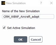
A New Simulation popup window appears. Enter CRM_WBNP_Aircraft_adapt to name the new simulation. Click OK to close the window. A new simulation called CRM_WBNP_Aircraft_adapt will be automatically loaded in Fluent Aero.
Go to the Input:Design Points table. Edit the Mach Number and the Angle of Attack [deg] columns of DP-2 with the values of 0.95 and 3.0 degree, respectively. Set the Status column of two DPs to Needs Update.

Note: The flight condition of DP-2 was modified to clearly observe the benefits of mesh adaption to capture shocks.
Click onto the Outline View → Setup. In the Setup panel, enable Mesh Adaption under Advanced Workflows
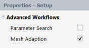
to reveal the Adaption node under the Solution tree of the Outline View.
Note: Fluent Aero conducts mesh adaption cycles per design point using PUMA with the Combined Hessian Indicator. At each design point, a baseline mesh solution is used to start the first adaption cycle.
Click on Solution → Adaption to set-up mesh adaption cycles. A cycle corresponds to a mesh adaption step, using the previous solution and its corresponding mesh, followed by a number of CFD solver iterations on the new adapted mesh.
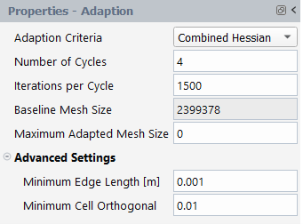
In the Properties – Adaption window,
Set the Number of Cycles to 4; the first cycle is used to obtain the baseline mesh solution.
Increase the number of Iterations per Cycle to 1500.
Reduce Advanced Settings → Minimum Edge Length [m] to 0.001 m.
Note: The Properties – Adaption window contain the following mesh adaption settings for PUMA.
Adaption Criteria:
The Combined Hessian Indicator is the default Error-based mesh adaption criteria of Fluent Aero. Other Hessian indicators are supported by selecting Case settings. These indicators should be defined inside the imported case file or via the Solution Workspace that is connected to Fluent Aero.
Number of Cycles:
This is the total number of adaption cycles to conduct per design point. Higher values will improve numerical precision but will result in larger mesh size.
Iterations per Cycle:
This is the number of RANS iterations per adaption cycle. This value times the number of cycles must be equal to the total number of iterations under the Solution --> Solve. As the number of cycles increases, more iterations per cycle are needed to fully converge a solution.
Baseline Mesh Size:
This is the mesh cell count of the baseline mesh. This mesh is the grid inside the imported case or mesh file used to create the simulation folder. The baseline mesh is automatically reloaded at the beginning of each design point.
Max.Adapted Mesh Size
This is the maximum number of cells that mesh adaption can produce. It sets an approximate limit to the total cell count of the mesh. The default value is zero and indicates that there is no mesh size constraint during mesh adaption.
Minimum Edge Length [m]
This is the minimum edge length of a cell to respect before refining it. A value of zero places no limit.
Minimum Cell Orthogonal
This the minimum cell orthogonal quality that the code attempts to maintain in the cells that results from adaption. The worse quality cells will have a value closer to 0 and better-quality cells will have a value closer to 1.
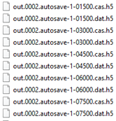
Go to Solution → Files in the Properties-Files window, enable Autosave Intermediate Solution Files, and set Save Solution Every (Iterations)to 1500.
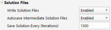
Note: Writing intermediate solutions allows you to inspect the adapted solutions at end of each mesh adaption cycle. To do this, the Save Solution Every (Iterations) must be equal to the Iteration per Cycle of the Properties – Adaption window. If Autosave Intermediate Solution Files is Disabled, only the final adapted solution is saved.
Go to Solution → Solve.
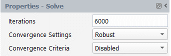
Set Iterations to
6000, which is equal to the Number of Cycles times Iterations per Cycle in the Adaption UI..Keep Convergence Settings to to improve convergence of the adapted meshes.
Disabel Convergence Criteria to let simulations run until the end of the 6000 iterations.
Click the button at the bottom of the Properties - Solve panel to start the mesh adaption calculations.
When conducting mesh adaption simulations in Fluent Aero, the baseline mesh file of the simulation is created from the imported case file. This mesh is then saved inside
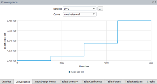
-baseline.cas.h5file and is located in the simulation folder. Fluent Aero will automatically reload the baseline mesh file at the beginning of each design point.During a mesh adaption simulation, the first adaption cycle consists in running an airflow solution on the baseline mesh. Then, at the beginning of the 2nd cycle, mesh adaption is carried out on the 1st cycle mesh using its solution. Mesh cells within the domain will be refined or coarsen based on the adaption’s predefined criteria. A new mesh is therefore generated and the previous solution is interpolated onto that mesh. Calculations will resume and continue until they reach their assigned number of iterations per cycle. This procedure is repeated until all adaption cycles have been ran. Since solutions are interpolated between adaption cycles, large fluctuations can be observed in the plots of Residual, lift/drag, and mesh cell count.
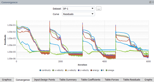
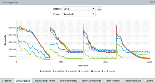
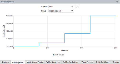
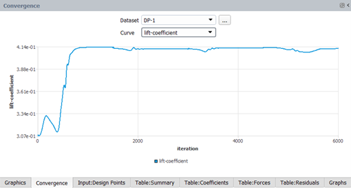
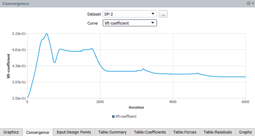
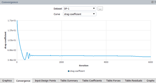
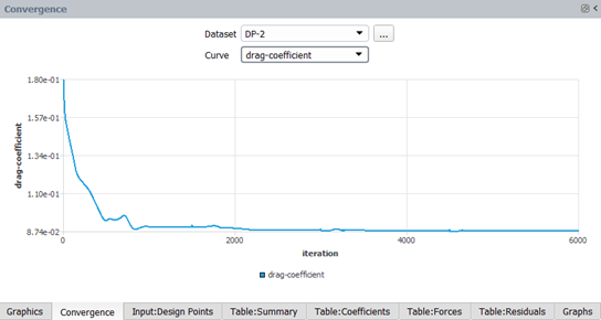
You can monitor the adaption simulation of each design point in the Convergence window on the right of your screen. The start of each adaption cycle can be easily observed by the jumps in Residual, lift-coefficient, and drag-coefficient plots. In addition, a mesh-size-cell curve can be used to monitor the size of the adapted meshes produced at each mesh adaption cycle. In this tutorial, the adaption events within the two design point’s simulations can be noticed at the iteration 1500th, 3000th, and 4500th in Figure 37.30: Residuals of DP-1 and DP-2, Figure 37.31: Mesh-size-cell of DP-1 and DP-2, Figure 37.32: Lift Coefficient of DP-1 and DP-2 and Figure 37.33: Drag Coefficient of DP-1 and DP-2.
Once your simulations are completed, go to the simulation
Resultfolder. You can find the intermediate adapted case and data files by right clicking the Results folder of your simulation located in the Project View. Select Open in File Explorer, to see these files.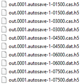
Go to the Convergence window. Set Dataset to DP-1 and then DP-2 and observe their Residual, mesh-size-cell, lift-coefficient, and drag-coefficient history by selecting these options next to Curve.
From the above figures, good residual convergence is maintained thought out the entire mesh adaption process. Moreover, aerodynamic coefficients seem to converge towards a unique solution that is different than the baseline solution, for instance DP-2.
The table below lists the values of lift and drag coefficients at each adaption cycle of DP-1 and DP-2.
Table 37.2: Lift and Drag Coefficients at each Adaption Cycle of DP-1
DP-1 1500th iteration 3000th iteration 4500th iteration 6000th iteration CL
(Lift-Coefficient)0.414004 0.412024 0.413293 0.412402 ∆CL – 0.00198 0.001269 0.000891 CD
(Drag-Coefficient)0.0492498 0.0487949 0.0481726 0.0452606 ∆CD -- 0.0004549 0.0006223 0.002912 Table 37.3: Lift and Drag Coefficients at each Adaption Cycle of DP-2
DP-1 1500th iteration 3000th iteration 4500th iteration 6000th iteration CL
(Lift-Coefficient)0.47618 0.424414 0.417245 0.409821 ∆CL – 0.052104 0.007169 0.007424 CD
(Drag-Coefficient)0.0899977 0.0881025 0.0877974 0.0876547 ∆CD -- 0.0018952 0.0003051 0.0001427 The above table confirms the trend observed in the Convergence plots as lift and drag coefficients converge towards a unique solution and their differences (∆CL and ∆CD) between adaption cycles decrease.
Note: DP-1 is a transonic condition. Its mesh adaption simulation requires more cycles to converge all aerodynamic coefficients.
In Project View , right-clickout.0002.cas.h5 located under Results→DP-2 and select Load Case to load the final adapted mesh of DP-2. In the similar way, right-click onto out.0002.dat.h5 and select Load to load the final adapted airflow solution of DP-2.
You can create graphics to quickly post-process the final adapted mesh and airflow solution of DP-2 from the Results node under the Outline View.
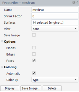
Click on Meshes under Graphics, then click New in the Properties – Meshes panel to create a new mesh display object mesh-1. Click on mesh-1 and do the following under its properties panel:
Change the Name to mesh-ac.
Set Surfaces to Wall type so that all walls of the CRM aircraft are selected.
Ensure that Options → Faces is enabled. Disable Nodes and Edges.
Click Display in the properties panel to show the aircraft in the Graphics window.
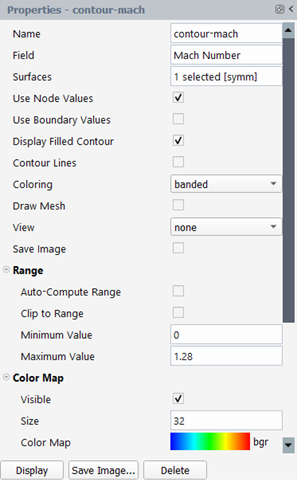
Right-click on Contours under Graphicsand select New to create a new contour-1 object. In the Properties panel of contour-1, do the following:
Change the Name to contour-mach.
Set Field to Mach Number.
Set Surfaces to Symmetry type to select the symmetry plane.
Set Coloring to banded.
Disable Auto-Compute Range under Range. Set Minimum Value and Maximum Value to 0 and 1.28, respectively.
Under Color Map,
Set Size to 32.
Set Color Map to bgr
Click Display in the properties panel to show the aircraft in the Graphics window.
Under Results → Design Point, right-click on Scene then select New to create a scene object.
Click on the new scene-1 object under Scene.
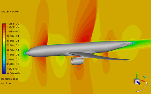
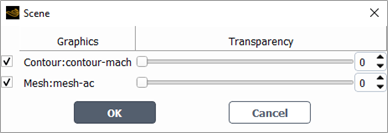
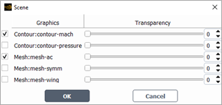
In Properties – scene-1 panel, click the text box next to Graphics Objects to bring up the Scene window. Then enable Contour: contour-mach and Mesh:mesh-ac under Graphics column. Click OK to close the window.
Click Display at the bottom of the Properties – scene-1 panel. The output view of scene-1 is displayed in the UI’s Graphics window.
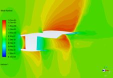
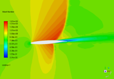
The figure above shows the Mach number field at the symmetry plane of the final adapted airflow solution of DP-2. Since the incoming airflow of DP-2 is close to sonic conditions, Mach 0.95, airflow reaches sonic speed after being accelerated by the aircraft’s geometry. Shocks as well as their locations are precisely captured over the fuselage.
You can also display the final adapted mesh of DP-2 by following these steps:
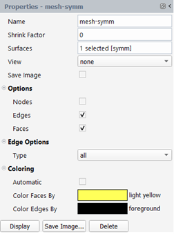
Click on Meshes under Graphics, then click New in the Properties – Meshes panel to create a new mesh display object mesh-1. Click on mesh-1 and do the following under its properties panel:
Change the Name to mesh-symm.
Set Surfaces to Symmetry type so that the symmetry plane is selected.
Ensure Options → Edges and Faces are enabled. Disable Nodes.
Under Coloring, disable Automatic. Set Color Faces By to light yellow and set Color Edges By to foreground.
Click Display in the properties panel to update mesh-symm settings.
Click on the scene-1 object under Scene tree node.
In Properties – scene-1 panel, click on the text box next to Graphics Objects to bring up the Scene window again. Disable Contour: contour-mach under Graphics column. Enable Mesh:mesh-ac and Mesh:mesh-symm under Graphics column. Click OK to close the window.
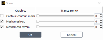
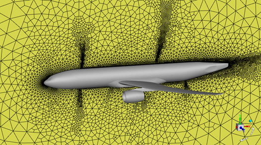
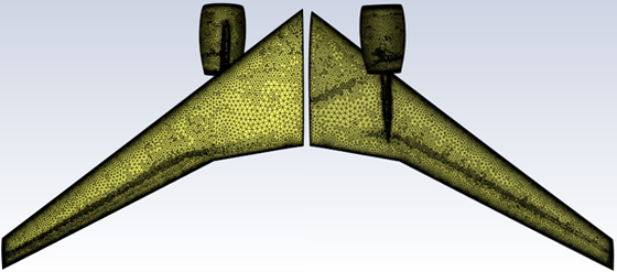
Click Display at the bottom of the Properties – scene-1 panel. The output view of scene-1 is displayed in the UI’s Graphics window as below.
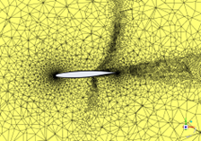
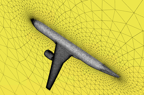
The above figure shows the extra mesh refinement, that was added to the baseline mesh by mesh adaption, to capture the most salient features of the solution Figure 37.35: Adapted Mesh on Symmetry Plane of DP-2’s Solution at the Last Adaption Cycle, such as shocks, wakes and the boundary layer over the fuselage.
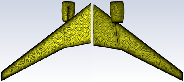
Right-click onto the mesh-symm object then select Copy to create another graphic mesh object. In the property panel of the new mesh object, set its Name as mesh-wing. Click on the selection box of Surfaces and ensure that only the walls of the engine and wing are selected. Click Display to view the surface mesh over the wing and engine in the Graphics window as Figure 37.36: Surface Mesh over the Wing of DP-2 at the Last Adaption Cycle (Adapted Mesh: Top=left , Bottom=right) below.
Figure 37.36: Surface Mesh over the Wing of DP-2 at the Last Adaption Cycle (Adapted Mesh: Top=left , Bottom=right)
Mesh adaption automatically refines the baseline surface mesh (Figure 37.36: Surface Mesh over the Wing of DP-2 at the Last Adaption Cycle (Adapted Mesh: Top=left , Bottom=right)) to capture the shock locations over the suction and pressure side of the wing. This allows for a precise representation of the pressure distribution [Figure 37.38: Surface Pressure over the Wing of DP-2’s Solution at the Last Adaption Cycle (Top=left , Bottom=right)] along the wing and consequently of the aerodynamic coefficients.
Figure 37.37: Surface Mesh over the Wing of DP-2 at the First Adaption Cycle (Baseline Mesh: Top=left , Bottom=right)
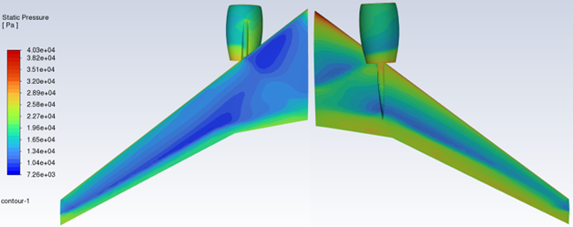
Right-click onto the contour-mach object then select Copy to create another graphic mesh object. In the property panel of the new mesh object, set its Name as contour-pressure. Change Field from Mach Number to Static Pressure. Click on the selection box next to Surfaces and ensure that only walls are selected except for the fuselage walls. Enable Auto-Compute Range under Range. Click Display to view the surface pressure over the wing and engine in the Graphics window as Figure 37.38: Surface Pressure over the Wing of DP-2’s Solution at the Last Adaption Cycle (Top=left , Bottom=right) below.
Figure 37.38: Surface Pressure over the Wing of DP-2’s Solution at the Last Adaption Cycle (Top=left , Bottom=right)
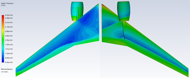
in the above image, the location of the shocks over the wing surface is precisely captured with mesh adaption. The sharp static pressure increase after the shock is better represented by the adapted solution than by the baseline result, Figure 37.38: Surface Pressure over the Wing of DP-2’s Solution at the Last Adaption Cycle (Top=left , Bottom=right). This is mainly due to the extra surface mesh refinement generated by the Combined Hessian Indicator as seen in Figure 37.36: Surface Mesh over the Wing of DP-2 at the Last Adaption Cycle (Adapted Mesh: Top=left , Bottom=right).
Figure 37.39: Surface Pressure over the Wing of DP-2’s Solution at the First Adaption Cycle (Top=left , Bottom=right)
Note: Only the final adapted mesh and solution can be post-processed in Fluent Aero. Fluent Aero cannot load intermediate solution files, such as the *.cas and *.dat files produced by each mesh adaption cycle, in Results to post-process them. These intermediate files can be loaded in Fluent standalone mode. Therefore, Figures in Step 14 and Step 15 were generated inside Fluent.
You may need to examine the results of the airflow calculation within the domain. Go to Results → Design Point (DP-2 Loaded) → Surfaces. Under the Properties – Surfaces panel, click on New → Plane to create a new cutting plane. Click onto plane-1 object. Set Creation Mode to XY Plane and Z [m] to 9.7. Go back to Surfaces and create a new plane. This new plane should be plane-2. Click onto this plane in the Outline View and set Creation Mode to XY Plane and Z [m] to 20. In this manner, you created two planes. The first plane, plane-1, cuts through the engine’s location while the second plane, plane-2, is located near the wing tip.
To display mach number over the cutting plane-1. Click on contour-mach under Contours, and set its Surfaces to plane-1. Enable Range → Auto-Compute Range and Use Global Range. Then, go to Scene→ scene-1 object → Graphisc Objects. Ensure the contour-mach and mesh-ac are enabled. Click Display.
Repeat the same step to display the Mach number on plane-2. The Mach number contours of plane-1 and plane-2 are shown in the figure below.
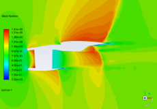
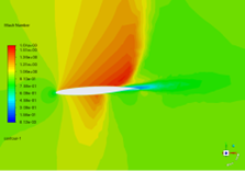
Figure 37.40: Mach Number over the Wing of DP-2’s Solution at the Last Adaption Cycle (Z = 9.7 on the Left and 20 m on the Right)
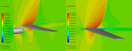
Shocks over the wing and nacelle and at the exhaust are sharply captured by mesh adaption. In addition, the wake produced by the wing and the flow generated by the exhaust are well resolved via mesh adaption.
You can also postprocess the adapted mesh and solutions from each adaption cycle to track how mesh adaption improves the airflow solution. Below are some images of how the mesh is adapted at each mesh adaption cycle and how the solution improves. Several flow features become more apparent with mesh adaption. For instance:
the shock produced by the exhaust and its interaction with the shear layer that originates from the lip of the nozzle
the shocks around the nacelle and on the pressure and suction sides of the wing are clearly visible on the last adapted mesh as this mesh received extra refinement to properly capture the pressure jump across these shocks
the wakes produced by the wing and nacelle.
Table 37.4: Meshes and Airflow Solutions of DP-2 over the Engine at Each Adaption Cycle (Z = 9.7 m)
Adapted Mesh Adapted Solution (Mach Number) Iteration 1500th
(1st Cycle with the baseline mesh)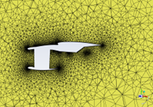 -
-
Iteration 3000th
(2nd Cycle)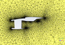
Iteration 4500th
(3rd Cycle)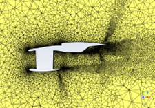
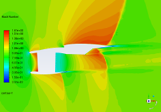
Iteration 6000th
(4th Cycle)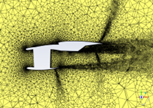
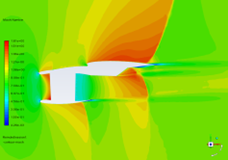
Table 37.5: Meshes and Airflow Solutions of DP-2 over the Wing at Each Adaption Cycle (Z = 20 m))
Adapted Mesh Adapted Solution (Mach Number) Iteration 1500th
(1st Cycle with the baseline mesh)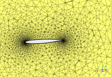 -
-
Iteration 3000th
(2nd Cycle)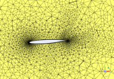
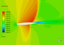
Iteration 4500th
(3rd Cycle)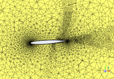
Iteration 6000th
(4th Cycle)