


As described in Connecting Systems in Workbench, systems in Workbench can easily be connected to each other and configured to perform a multitude of physics-based simulations and analyses.
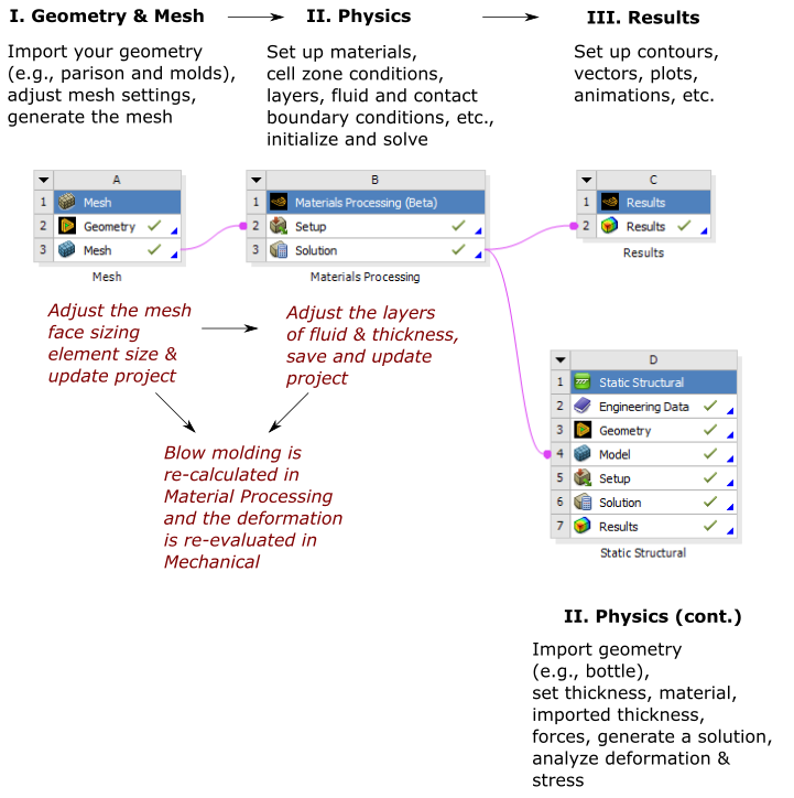
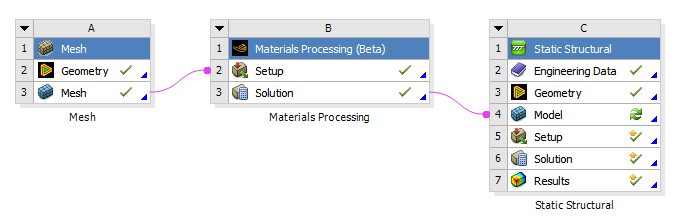
This section provides a walk through of setting up solving a 3D blow molding simulation of a bottle in Workbench involving a Mesh system, a Materials Processing system (Fluent Materials Processing Workspace), a Results system, and a Static Structural system. The Static Structural system allows you to check the resistance of the blown product.
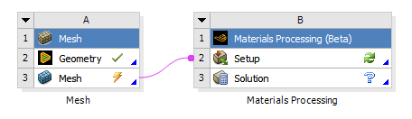
Figure 34.1: Configuring the Materials Processing System with a Mesh and a Results System and a Static Structural System
This tutorial is divided into the following sections:
This tutorial demonstrates how to do the following:
Launch Ansys Workbench.
Create an Ansys Meshing component system in Ansys Workbench.
Import the parison/mold geometry
Create the computational mesh for the geometry using Ansys Meshing.
Create a Materials Processing workspace component system in Ansys Workbench.
Set up and solve the CFD simulation in the Materials Processing workspace.
Create a Results component system in Ansys Workbench and analyze the results in CFD-Post.
Create a Static Structural component system in Ansys Workbench and analyze the resistance of the blown product.
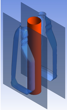
This tutorial simulates a typical blow molding situation for a bottle. In the present case, it is assumed that a cylindrical parison with uniform thickness distribution has been extruded. The present calculation involves two major steps; parison pinch-off due to mold closing, and inflation. Figure 34.2: Blow Molding Initial Configuration shows a sketch of the process in the initial configuration, before the pinch-off and parison inflation.
From a geometric point of view, the initial parison has the following dimensions:
height = 0.276 m
radius = 0.0225 m
initial thickness = 0.003 m
The thickness of the fluid parison is much smaller than the other two dimensions of the bottle, which allows for the use of the membrane (shell) element, which is suited for the analysis of 3D blow molding simulations. It is important to remember when preparing the surface mesh, that the mesh elements on the mold should not be the same order of magnitude as the expected final local thickness. The use of the membrane element is presently restricted to time-dependant flows and is combined with Lagrangian representation. That is, each mesh node is a material point.
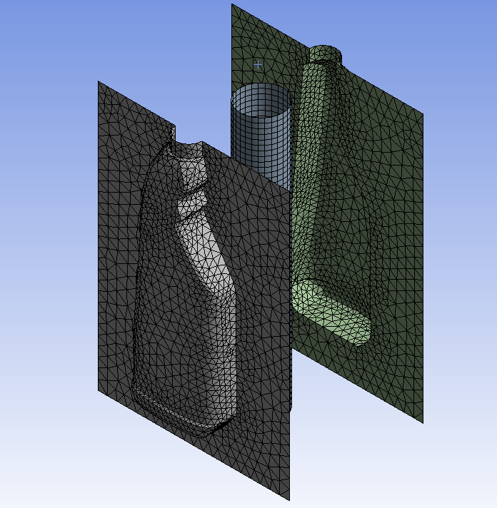
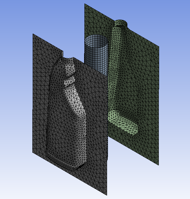
The finite element mesh and the boundary conditions are displayed in Figure 34.3: Finite Element Mesh, Subdomains, and Boundary Sets. As shown, a full 3D finite element is built for both the mold and the parison. Only a surface mesh is needed for both the mold and the parison, but the most important aspect remains the proper description of the inner mold surfaces that will shape the bottle.
The parison has the following material properties in SI units:
model: shell model, Gen. Newtonian isothermal
viscosity = 104 Pa s
density = 900 kg/m3
inertial terms taken into account
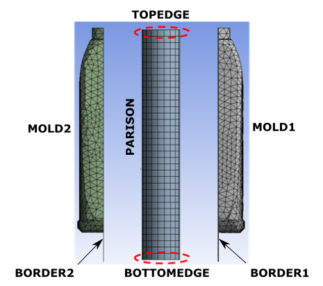
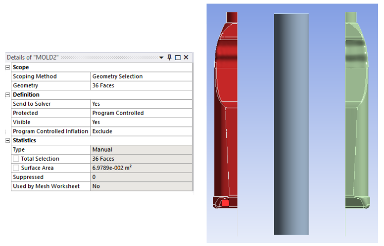
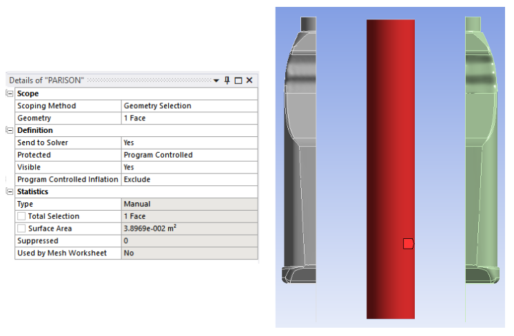
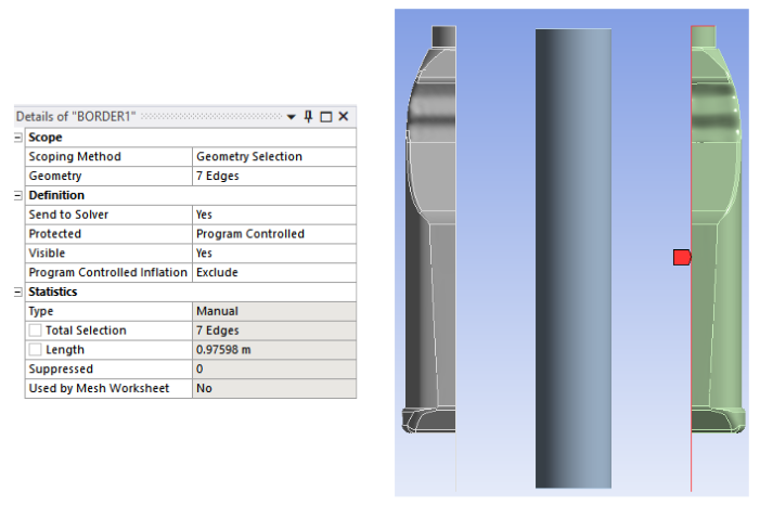
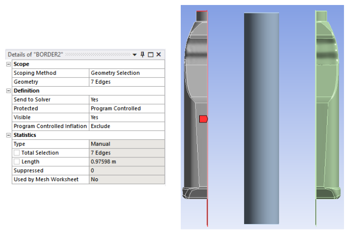
As seen in Figure 34.3: Finite Element Mesh, Subdomains, and Boundary Sets, the mesh topology involves three subdomains (MOLD2, PARISON, and MOLD1) and two boundary sets (TOPEDGE and BOTTOMEDGE). The edges of MOLD1 and MOLD2 are designated by BORDER1 and BORDER2, respectively. The fluid parison is covered by the subdomain named PARISON while MOLD2 and MOLD1 will be defined as molds. Along boundary sets TOPEDGE and BOTTOMEDGE, a symmetry boundary condition will be imposed. The inflation pressure will be defined on the subdomain representing the parison.
The following sections describe the setup and solution steps for this tutorial:
To prepare for running this tutorial:
Prepare a working folder for your simulation.
Download the
workbench_matpro_blowmold.zipfile here .Unzip the
workbench_matpro_blowmold.zipfile you have downloaded to your working folder.Two geometry files (
bottle.agdbandparison+molds.agdb) can be found in the unzipped folder.Start Workbench from .
Create a Mesh component system by drag and drop in Workbench.
Import a geometry file into the Geometry cell.
For this tutorial, we'll use a geometry file (
parison+molds.agdb) that contains the parison and both molds.Double-click the Mesh cell to open Ansys Meshing, and make the following changes.
Select the Mesh in the tree.
Set general mesh properties.
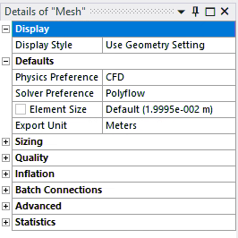
For the Physics Preference, select CFD.
For the Solver Preference, select Polyflow.
For the Export Unit, select Meters.
Create a face meshing object for the tube parison.
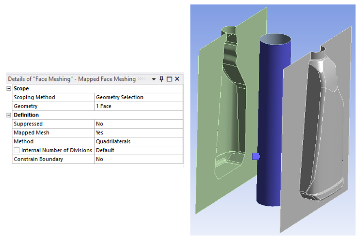
Right-click the Mesh in the tree and insert a Face Meshing object.
Select the tube parison as the Geometry.
Create a sizing object for the tube parison.
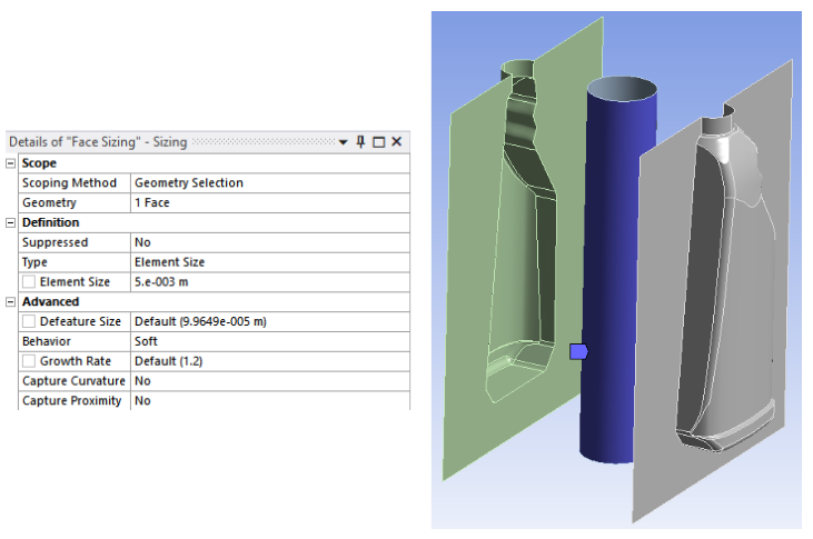
Right-click the Mesh in the tree and insert a Sizing object.
Select the tube parison as the Geometry.
Set the Element Size to
0.005m.
Create a method object for the left mold.
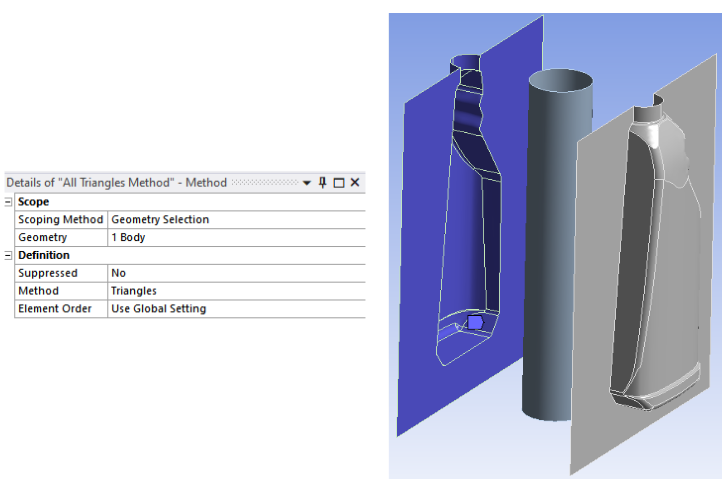
Right-click the Mesh in the tree and insert a Method object.
Select the left mold as the Geometry.
Set the Method to Triangles..
Create a duplicate method object for the right mold.
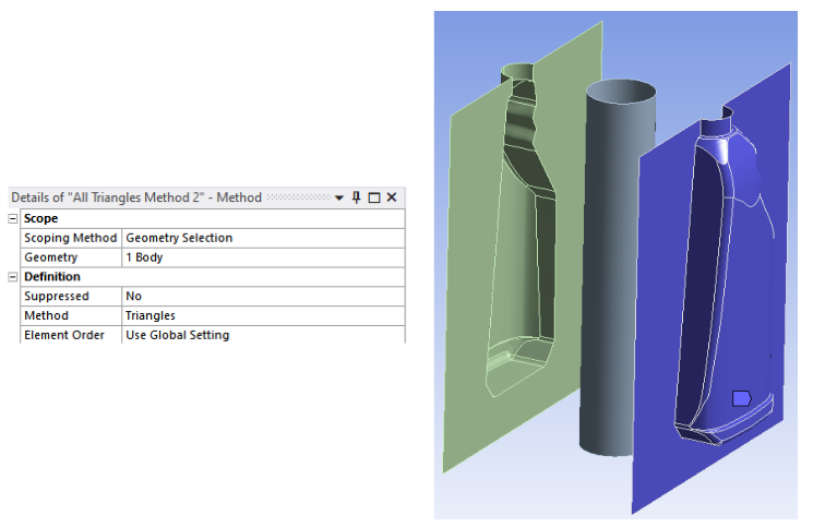
Right-click the new All Triangles method in the tree, and duplicate it.
Select the right mold as the Geometry.
Create another sizing object for the right mold.
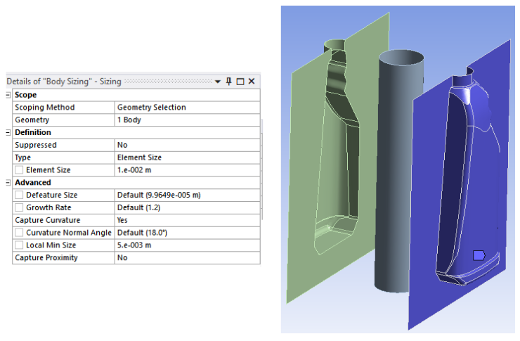
Right-click the Mesh in the tree and insert another Sizing object.
Select the right mold as the Geometry.
Set the Element Size to
0.01m.Set the Capture Curvature to Yes.
Set the Local Min Size to
0.005m
Create a duplicate sizing object for the left mold.
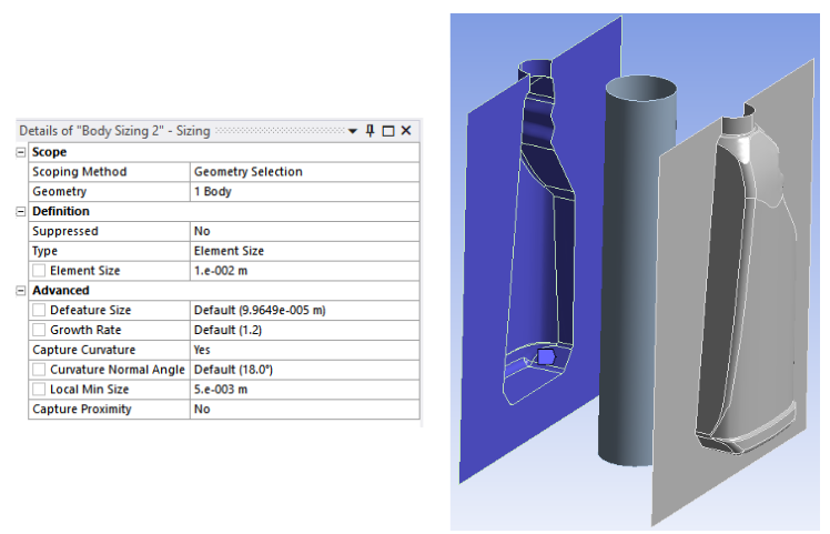
Right-click the new Body Sizing object in the tree, and duplicate it.
Select the left mold as the Geometry.
Generate the mesh by right-clicking the Mesh in the tree and select the Generate Mesh option (or use the Ribbon).
Create named selections.
When viewed from the +X axis, select all faces of the right mold, right-click the selected faces and select Create Named Selection..., assigning the name of MOLD1.
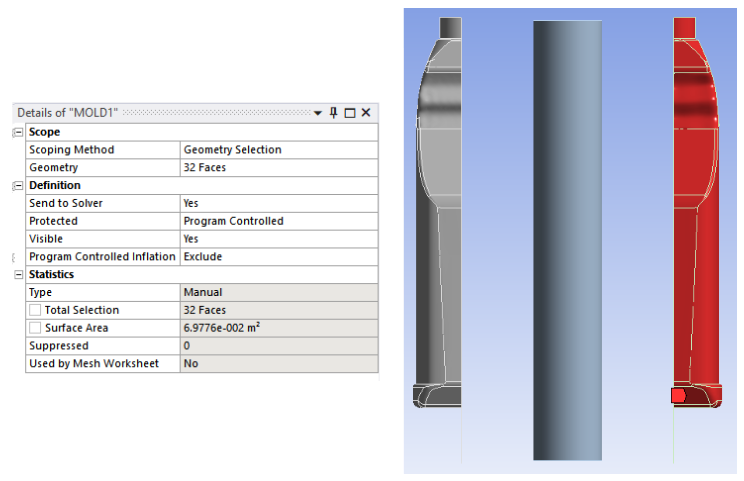
When viewed from +X axis, select all faces of the left mold, right-click the selected faces and select Create Named Selection..., assigning the name of MOLD2.
Select the tube of the parison, right-click the selected face and select Create Named Selection..., assigning the name of PARISON.
When viewed from +X axis, select all bordered edges of the right mold, right-click the selected edges and select Create Named Selection..., assigning the name of BORDER1.
When viewed from +X axis, select all bordered edges of the left mold, right-click the selected edges and select Create Named Selection..., assigning the name of BORDER2.
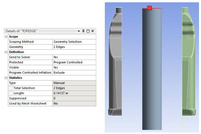
Select the top edges (max Y) of the tube parison, right-click the selected edges and select Create Named Selection..., assigning the name of TOPEDGE.
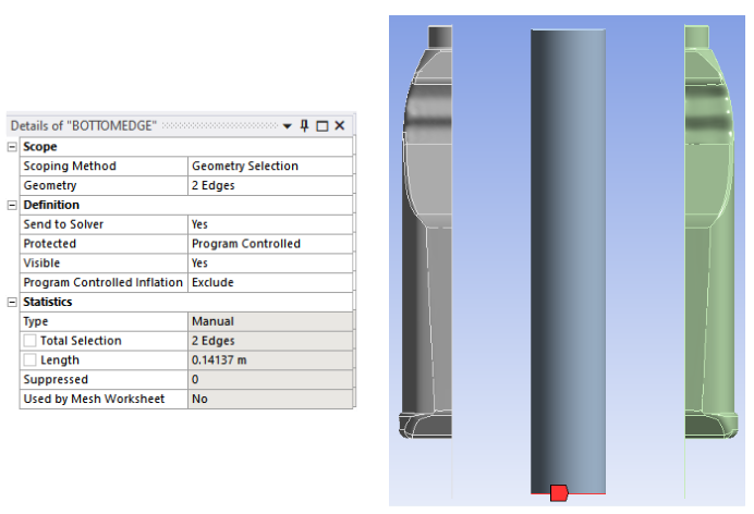
Select the bottom edges (min Y) of the tube parison, right-click the selected edges and select Create Named Selection..., assigning the name of BOTTOMEDGE.
Right-click Mesh in the tree, and select Update in the context menu.
Close the Ansys Meshing application.
Create a Materials Processing component system by drag and drop in Workbench, connecting to the Mesh cell of the Mesh system.
Right-click the Mesh cell and select Update.
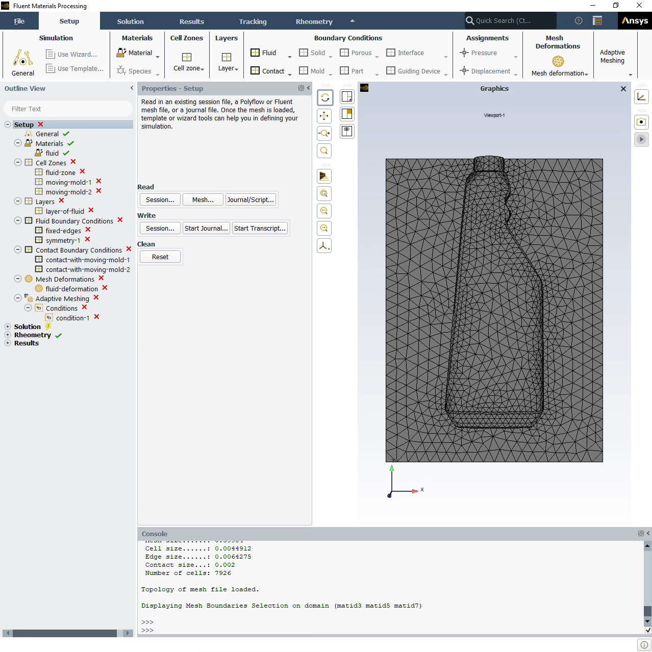
Edit the Setup cell in the Materials Processing component system to open the Fluent Materials Processing workspace.
Create a blow molding simulation using a template.
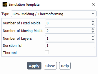
Click Use Template... in the Ribbon.
 Setup
→ Simulation →
Use Template...
Setup
→ Simulation →
Use Template...
Set the Type to Blow Molding / Thermoforming.
Set the Number of Moving Molds to
2.Click Apply.
Set material properties for the fluid (fluid).
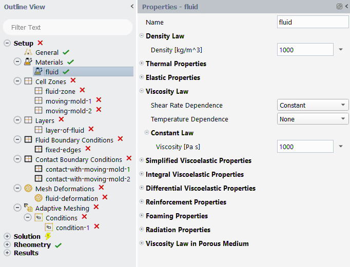
In the Outline View, select fluid to see it's properties in the Properties Window.
Set the Density to
1000kg/m3.Set the Viscosity to
10000Pa s.
Set cell zone properties for the fluid (fluid-zone).
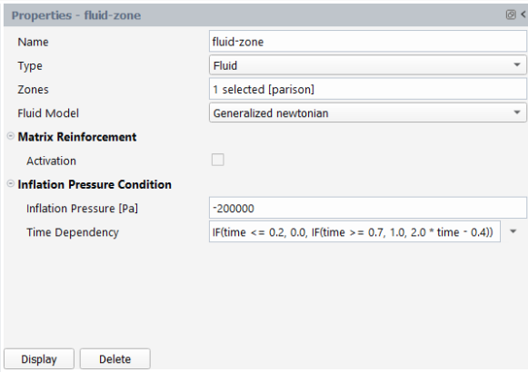
In the Outline View, select fluid-zone to see it's properties in the Properties Window.
For Zones, select parison.
Set the Inflation Pressure to
-200000Pa s.Select expression from the Time Dependency drop-down list, then enter
IF(time <= 0.2, 0.0, IF(time >= 0.7, 1.0, 2.0
                                        * time - 0.4))
for the time dependency.Click Display.
Arrows will indicate the pressure acting from the inside the tube parison towards the exterior in order to inflate it.
Set cell zone properties for the first moving mold (moving-mold-1).
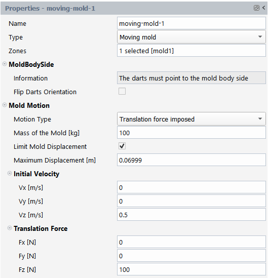
In the Outline View, select moving-mold-1 to see it's properties in the Properties Window.
For Zones, select mold1.
For Motion Type, select Translation force imposed.
Set the Mass of the Mold to
100kg.Enable the Limit Mold Displacement option, and set the Maximum Displacement to
0.06999m.Set the Initial Velocity Vz to
0.5m/s.Set the Translation Force Fz to
100N.
Set cell zone properties for the second moving mold (moving-mold-2).
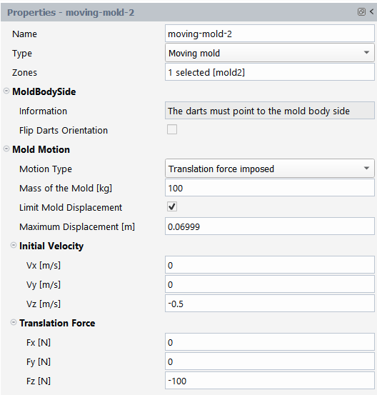
In the Outline View, select moving-mold-2 to see it's properties in the Properties Window.
For Zones, select mold2.
For Motion Type, select Translation force imposed.
Set the Mass of the Mold to
100kg.Enable the Limit Mold Displacement option, and set the Maximum Displacement to
0.06999m.Set the Initial Velocity Vz to
-0.5m/s.Set the Translation Force Fz to
-100N.
Define the layer (layer-of-fluid).
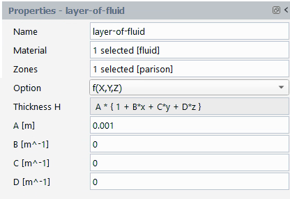
In the Outline View, select layer-of-fluid to see it's properties in the Properties Window.
For Zones, select parison.
Set the value of A to
0.001m.
Delete the unnecessary fluid boundary condition (fixed-edges). Right-click fixed-edges, and select Delete from the context menu.
Define a symmetry boundary condition (symmetry-1).
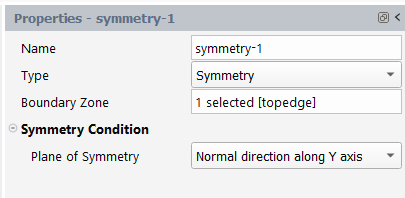
In the Ribbon, click Setup > Boundary Conditions > Fluid > New > Symmetry.
For Boundary Zone, select topedge.
For Name, specify symmetry-1.
Select Normal direction along Y axis.
Define another symmetry boundary condition (symmetry-2).
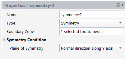
In the Ribbon, click Setup > Boundary Conditions > Fluid > New > Symmetry.
For Boundary Zone, select bottomedge.
For Name, specify symmetry-2.
Select Normal direction along Y axis.
Define the first contact boundary condition (contact-with-moving-mold-1).
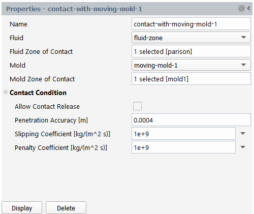
In the Outline View, select contact-with-moving-mold-1 to see it's properties in the Properties Window.
For Fluid Zone of Contact, select parison.
For Mold Zone of Contact, select mold1.
Enter
1e9for the Slipping Coefficient.Enter
1e9for the Penalty Coefficient.
Define the second contact boundary condition (contact-with-moving-mold-2).
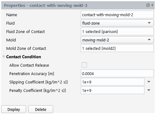
In the Outline View, select contact-with-moving-mold-2 to see it's properties in the Properties Window.
For Fluid Zone of Contact, select parison.
For Mold Zone of Contact, select mold2.
Enter
1e9for the Slipping Coefficient.Enter
1e9for the Penalty Coefficient.
Define the mesh deformation (fluid-deformation).
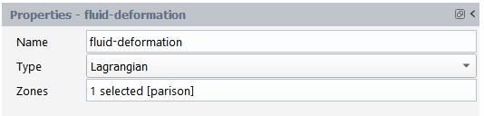
In the Outline View, select fluid-deformation to see it's properties in the Properties Window.
For Zones, select parison.
Disable adaptive meshing.
In many practical cases, the use of adaptive meshing based on contact, remeshing, or both may be useful to selectively and automatically refine the mesh during the solution. The blow molding simulation template automatically includes adaptive mesh refinement, however, it is not necessary for this tutorial.
In the Outline View, select Adaptive Meshing to see it's properties in the Properties Window.
Deselect the Enabled check box.
Specify output settings:
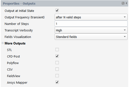
In the Outline View, select Solution > Outputs.
Under More Outputs, enable Ansys Mapper.
Check the setup and perform the calculations.
In the Outline View, select Solution > Run Calculation.
Click the Check button.
Click the Calculate button.
Check for convergence in the listing file, available next to the graphics window in the Listing tab. It is a common practice to confirm that the solution proceeded as expected by looking for the following printed at the bottom of the listing file:
The computation succeeded.
Check for convergence using residual plots, available next to the graphics window in the Plots tab.
Go to File > Exit to close the workspace.
Confirm that you want to quit the application, and confirm that you want to save the session.
Use Mechanical to further study the Materials Processing simulation.
Create a Static Structural analysis system by drag and drop in Workbench.
Import the
bottle.agdbgeometry file into the Static Structural system.Connect to the Solution cell of the Materials Processing system to the Model cell of the Static Structural system.
Edit the Model Cell in the Static Structural analysis system to open Mechanical.
Set material properties for the bottle's surface body.
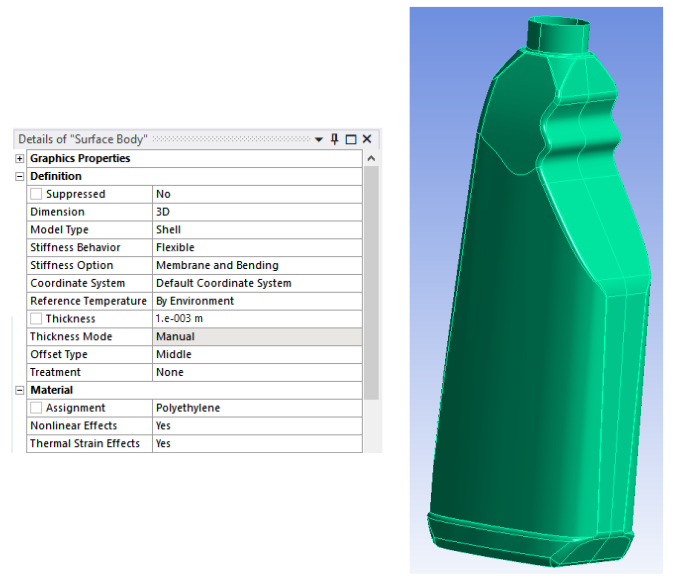
In the Outline View, select Geometry > Surface Body.
Set the Thickness to
0.001m.Set the Assignment to Polyethylene.
Set thickness properties for the bottle's surface body.
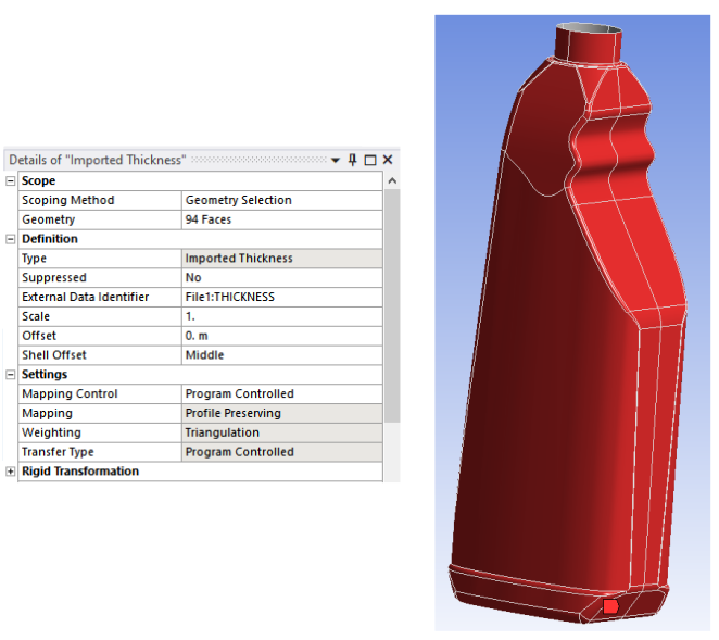
In the Outline View, select Geometry > Imported Thickness > Imported Thickness.
Select all faces of the geometry.
Click Scope > Geometry > Apply.
Right-click Geometry > Imported Thickness > Imported Thickness and select Import Thickness.
After import, the thickness is visible on the geometry.
Create a fixed support.
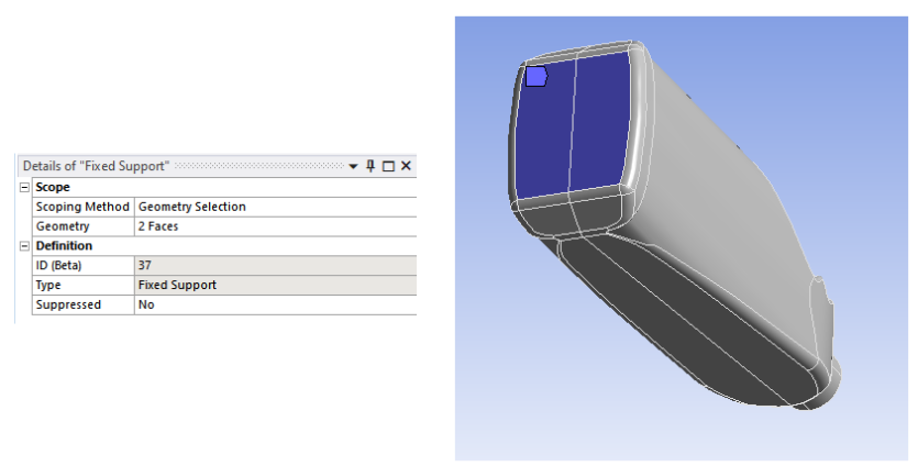
In the Outline View, right-click Static Structural, choose Insert > Fixed Support and select the two faces at the bottom of the bottle geometry.
Click Scope > Geometry > Apply.
Create a force.
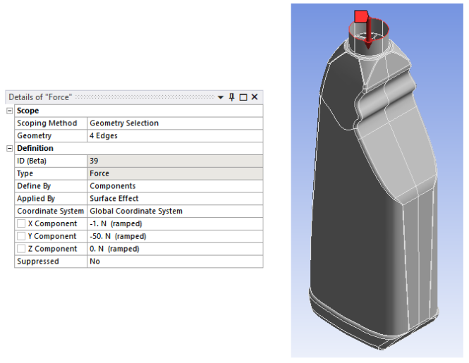
In the Outline View, right-click Static Structural, choose Insert > Force and select the four edges at the top of the bottle geometry.
For Define By, select Components.
For X Component, specify
-1N.For Y Component, specify
-50N.
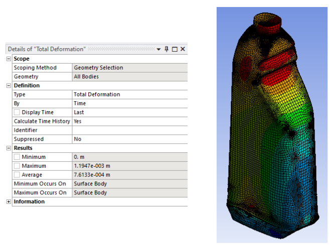
Create a total deformation solution object by right-clicking Solution and choosing Insert > Deformation > Total.
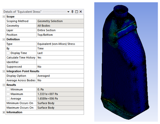
Create an equivalent stress solution object by right-clicking Solution and choosing Insert > Stress > Equivalent (von-Mises).
Click Solve.
Analyze the results.
Click Solution > Total Deformation.
Click Solution > Equivalent Stress.
Click Graph > Animation > Play.
Click Graph > Animation > Stop.
Edit the Mesh cell in the Mesh system.
Click Mesh > Face Sizing and change the Element Size to
0.004m.Click Update Project in Workbench to update the project.
The blow molding is re-calculated in the Materials Processing system and the bottle deformation is re-evaluated in Mechanical
Edit the Setup cell in the Materials Processing system.
Click Setup > Layers > layer-of-fluid and change A to
0.0015m.Click File > Exit.
Confirm that you want to quit the application, and confirm that you want to save the session.
Click Update Project in Workbench to update the project.
The blow molding is re-calculated in the Materials Processing system and the bottle deformation is re-evaluated in Mechanical
This tutorial introduced using the Fluent Materials Processing workspace within Workbench while analyzing a parison blow molding problem via Mechanical. The two halves of the mold moved into contact with the parison, where it became pinched, and a vacuum was applied to the parison. This blew the parison into the mold where it assumed the shape of the mold, which was a bottle in this case.
You represented the parison by a shell geometry under the valid assumption that the thickness of the parison was much smaller than the other two dimensions (diameter and height). The Materials Processing workspace used Polyflow to linearly interpolate the process variables—thickness, velocity and position. As a separate exercise, you could employ CFD-Post to report the individual time steps and view the thickness of the product as a function of time, or you can use the transient postprocessing capabilities within the workspace.