


This section describes the following topics:
Analyzing the results provided by a simulation may be challenging, especially if the flow occurs in a complex geometry, if it is transient, or if we want to compare results obtained with similar setups. How can we render our analysis “objective”? In this chapter, we propose a set of tools to reach that goal, and more specifically, tools to quantify the various aspects of the mixing process.
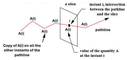
The basic idea is the following: we release in the flow domain a large set of material points (also named massless or virtual particles) and compute their pathlines in the flow. Along these pathlines, we evaluate and store in files a set of relevant quantities (temperature, velocities, shear-rate, ..). Once this “tracking” task is completed for a large set of points, we perform a statistical analysis on these quantities: we cut these pathlines at various times (if the flow is transient) or by cutting planes (if the flow has inlet and outlet sections): each slice will thus contain a sample of values (E.G. all temperatures of pathlines crossed by plane z=3). For each sample, we can evaluate mean, standard deviation, histograms, etc., leading to a quantified and objective measurement of some characteristics of the flow (e.g. residence time distribution at the outlet section of the flow domain, time evolution of the axial distribution of points in an extruder, fraction of points experiencing a stress above a given threshold, ..).
In polymer blending, a minor component is generally present as drops (or filaments) in a continuous phase of a major component. Mixing is a process of deformation and rupture of the drops but also a process of distribution of those drops in the whole flow domain. Good mixing is characterized by small and identical drops distributed uniformly throughout all of flow domain.
Deformation of drops is promoted by the viscous stress  exerted on the drops by the flow field and counteracted by the
interfacial stress
exerted on the drops by the flow field and counteracted by the
interfacial stress  .
.  is the interfacial tension and R, the local radius. The capillary
number is useful to characterize mixing.
is the interfacial tension and R, the local radius. The capillary
number is useful to characterize mixing.

For a given pair of polymers, a critical Capillary number may be found. It corresponds to the situation where the viscous stress competes with the interfacial stress. The drop is extended and finally breaks up into smaller droplets. This process is called dispersive mixing. Note that an extensional flow field is more efficient for breaking up drops into droplets than a shear flow is.
If the capillary number is much higher than the critical capillary number, then the viscous stress overrules the interfacial stress, and the drop is extended but does not break up. This process is called distributive mixing. Conversely, if the capillary number is much lower than the critical capillary number, then the interfacial stress dominates, and the drop is only slightly deformed.
In general, mixing begins with a distributive step (drops are deformed passively), followed by a dispersive step (drops break up into droplets), and finally by the distribution of the droplets in the flow. The following paragraphs focus on distributive mixing (Kinematic Parameters) and on distribution of material points into the flow domain (Distribution Mixing). A short paragraph presents also the quantities that can be used to evaluate the dispersive mixing.
One way to measure distributive mixing is to quantify the capacity of the flow to deform matter and to generate interface.
For 2D flows, the interface between fluids is a line. Instead of calculating the evolution of this interface (a very complex and impossible task to perform because of the exponential growth of the interface), the stretching of infinitesimal vectors attached to a large number of material points distributed in all the flow domain is calculated. As the points move in the flow, the vectors are stretched. The stretching and the rate of stretching of these vectors are properties that vary by time and location in the flow domain. Statistical analysis of the results provide a global overview of the process. Using this method, you have an objective and quantitative evaluation of the mixing of any process. You can, for example, find areas of poor mixing in the domain (low stretching instead of exponential increase). For 3D flows, the interface is a surface and the stretching of infinitesimal surfaces attached to material points is calculated.
Let  and
and  denote the domain occupied by the homogeneous fluid at time 0
and
denote the domain occupied by the homogeneous fluid at time 0
and  , respectively. The motion of the fluid is described by the
relationship
, respectively. The motion of the fluid is described by the
relationship
 | (34–1) |
where  denotes the position of a material point
  in
in  and
and  in
in  . The symbols
  and
and  denote the deformation gradient and the right Cauchy Green
strain tensor between both configurations. The velocity gradient and the rate of
deformation tensor at time
denote the deformation gradient and the right Cauchy Green
strain tensor between both configurations. The velocity gradient and the rate of
deformation tensor at time  are denoted by
  and
and  , respectively. For later use, note that
 | (34–2) |
The dot denotes the material time derivative.
Kinematic Parameters for 2D Flows
Consider in  , a material fiber
  with a unit orientation
  which deforms into a material fiber
  with a unit orientation
  at time
  . With
  denoting the length stretch
  . It follows [4] that:

while  is given by
 | (34–3) |
Good mixing quality requires high values of  throughout time and space. A local evaluation of the
efficiency of mixing [5] is given by the ratio
throughout time and space. A local evaluation of the
efficiency of mixing [5] is given by the ratio
 | (34–4) |
where
 | (34–5) |
The values of this instantaneous efficiency are always included in the interval [-1; 1]. Through manipulation it follows:
 | (34–6) |
Note that  is a local measure along the path of a material point. The
time-averaged efficiency is defined as
is a local measure along the path of a material point. The
time-averaged efficiency is defined as
 | (34–7) |
The global efficiency over all of the material points initially distributed in the flow is defined as:
 | (34–8) |
This global efficiency is the ratio of the output—the mixing
obtained—(the total stretching of the matter until time  ) over the input—the "energy" —(the total
mechanical dissipation until time
) over the input—the "energy" —(the total
mechanical dissipation until time  ).
).
Kinematic Parameters for 3D Flows
For 3D flows, you can calculate the local stretching of infinitesimal surfaces
by the mean of the area stretch  .
.
In the initial configuration  , consider an infinitesimal surface
  with a normal direction
  . This surface deforms with time. At time
  , the surface is noted
  , with a new normal direction
  . The area stretch
  , is the ratio of the deformed surface
  at time
  over the initial surface
  .
.
 | (34–9) |
For an incompressible fluid:
 | (34–10) |
If the fluid is incompressible, the normal direction to the surface
is:
 | (34–11) |
A good mixing quality requires high values of  throughout time and space. A local evaluation of the
efficiency of mixing [5] is given by the ratio
throughout time and space. A local evaluation of the
efficiency of mixing [5] is given by the ratio
 | (34–12) |
The values of this instantaneous efficiency are always included in the interval [-1; 1]. After some transformations:
 | (34–13) |
Note that  is a local measure along the path of a material point; the
time-averaged efficiency is defined as
is a local measure along the path of a material point; the
time-averaged efficiency is defined as
 | (34–14) |
For 3D kinematic parameters, a global efficiency over all the material points initially distributed in the flow is defined:
 | (34–15) |
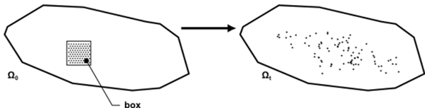
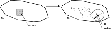
Suppose you want to distribute a cluster of particles initially concentrated in a small box (see figure below). It is assumed that the particles do not affect the flow field and that there is no interaction between them.
There exist several ways to quantify this process. Let us examine them one by one:
Distance distribution index:
The flow distributes this set of points as a function of time. We observe that the distance between points increase. It is important to define a distribution index to quantify this process. Its definition is based on the work performed by Manas-Zloczower and her colleagues [1], [2].
At time t, there are N points distributed in the flow domain.
Option 1: These points can form N(N-1)/2 pairs of points. For each pair of points xi and xj, their inter- distance
 is calculated. The maximum inter-distance will be
of the order of the diameter of the mixer.
is calculated. The maximum inter-distance will be
of the order of the diameter of the mixer. Option 2: The inter distance
 , between each point xi and its closest neighbour,
xj is
stored. Thus, we compute only N distances. Using this method of
calculation helps to better discriminate distributive capabilities
of similar mixers. The maximum inter-distance will be of the order
of
, between each point xi and its closest neighbour,
xj is
stored. Thus, we compute only N distances. Using this method of
calculation helps to better discriminate distributive capabilities
of similar mixers. The maximum inter-distance will be of the order
of  , where V is the volume of the mixer.
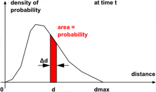
 With this set of distances, we can calculate the density of probability function on the distance f(d) : the probability to find a pair of points (chosen randomly) such that their inter-distance is included in range
 at time t is:
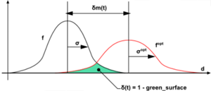
Now suppose you have randomly distributed the same number of points throughout the flow domain. You can assume that this is an ideal distribution. Using the same tools, you can calculate the function
 for this optimal distribution. It is noted
 .
.The distance distribution index,
 , is defined as the deviation of the function f(d)
(real distribution) from the function
, is defined as the deviation of the function f(d)
(real distribution) from the function  (optimal distribution):
As the distribution improves, the index
 decreases. This index is dimensionless — it
is independent of the size of the flow domain. The evolution of
decreases. This index is dimensionless — it
is independent of the size of the flow domain. The evolution of
 depends on the initial position of the box.
Another important parameter is the number or material points to
distribute; a careful analysis must be done to measure its influence.
depends on the initial position of the box.
Another important parameter is the number or material points to
distribute; a careful analysis must be done to measure its influence.distribution in zones
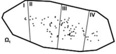
The distance distribution index is a global index, and thus it is unable to detect local defects (part of the mixer with a lack or an excess of points). Using this next method, you can detect such zones. As for the distance distribution index, we start with a cluster of particles initially concentrated in a small box (see figure above “Distributing massless particles from a small box”). It is assumed that the particles do not affect the flow field and that there is no interaction between them.
As a function of time, the flow distributes this set of points. The flow domain is partitioned into a set of adjacent and non-overlapping zones. In the figure below, as an example, we divided the flow domain in four zones:
The same number of points
 , is then distributed randomly throughout the flow
domain (it is assumed that this is the optimal distribution).
, is then distributed randomly throughout the flow
domain (it is assumed that this is the optimal distribution). One determines the number of points in each zone, for both distributions at time
 . Based on these numbers, one can evaluate a
relative error of distribution for each zone,
. Based on these numbers, one can evaluate a
relative error of distribution for each zone,  .
.
(34–16)
 is the number of points of the real distribution
included in zone
is the number of points of the real distribution
included in zone  , at time
  .
.  is the number of points of the optimal
distribution included in the same zone.
is the number of points of the optimal
distribution included in the same zone.If
 is zero for a zone, the optimal number of points
are in that zone.
is zero for a zone, the optimal number of points
are in that zone.If is negative for a zone, there is a lack of points in that zone as compared to the optimum.
If
 is positive for a zone, there are too many points
in that zone as compared to the optimum.
is positive for a zone, there are too many points
in that zone as compared to the optimum.A global index based on all the zones is defined as,

(34–17)
The number of points and the zone partitioning influences the indices described above. When comparing two different mixers, it is recommended that you keep the ratio number of points and zones constant. In order to have relevant results, this ratio should be higher than 100.
deviation of points concentration
As for the distance distribution index, the goal is to quantify distributive mixing. As for the previous parameters, there is a cluster of particles initially concentrated in a small box (see figure below).
As a function of time, the flow distributes this set of points.
At time t, there are N points distributed throughout the flow domain.
For each point xi, the number of neighbors xj, within a sample radius R are determined. Depending on the dimensionality (dim) of the cluster of points at time t, you can evaluate the local points concentration
 :
:
where Nx is the number of points of the cluster around xi at a distance smaller than the radius R.
With a perfect distribution of the points, the points are equally distributed throughout the entire flow domain. That is, there are the same number of points per unit volume found everywhere in the domain. The perfect points concentration
 , corresponds to the number of points divided by
the volume of the flow domain. You can adapt this method for
determining the perfect points concentration for other situations
(see § Points Concentration Deviation Function).
, corresponds to the number of points divided by
the volume of the flow domain. You can adapt this method for
determining the perfect points concentration for other situations
(see § Points Concentration Deviation Function).The standard deviation of points concentration at time
 is evaluated as
Where
 is the number of points in the cluster at time
 . xi corresponds to the
location of point
. xi corresponds to the
location of point  at time
  and
and  is the perfect points concentration.
Note that the points concentration is only evaluated at positions where there are points. There is no points concentration evaluation in zones of the mixer that do not contain material points. If distributive mixing improves, the points concentration deviation should decrease. At perfect distribution, the same points concentration is found at any location in the cluster, and the deviation is zero.
Dispersive mixing can also be analysed by adding postprocessors to the flow calculation:
Mixing index (or 'flow number') — indicates if the flow is locally a rigid motion (mixing index = 0), a shear flow (mixing index = 0.5), or in extension (mixing index = 1).
Stress — this field gives access to the stress magnitude in the direction of the local velocity (v.T.v) that stretches and breaks the drops.
Once the flow and those postprocessors are determined, you can calculate the evolution of the mixing index and the vTv stress component along the trajectories of material points. With these data you can evaluate the fraction of the matter experiencing a given stress value and evaluate the efficiency of the dispersive mixing.
Typically, trajectories are calculated by the time integration of the equation
 with a Euler explicit scheme. This method is sufficient when only
interested in the successive positions of material points. However, a more accurate
numerical technique is required if you want to precisely know how matter deforms
around material points as they travel the flow domain.
with a Euler explicit scheme. This method is sufficient when only
interested in the successive positions of material points. However, a more accurate
numerical technique is required if you want to precisely know how matter deforms
around material points as they travel the flow domain.
The tracking module combines two techniques using explicit fourth order Runge-Kutta and a coordinate transformation is performed instead of integrating the motion of a particle in the real space. The trajectory in the parent element is integrated with the Runge-Kutta method.
 | (34–18) |
Successive positions of the particle in real space are calculated using:
 | (34–19) |
The tracking module algorithm is as follows:
Initialization
Find the element
 , which contains the initial position
 .
. Find the local coordinates,
 , of
, of  in element
  .
.
The algorithm solves using the following loop unless a stop is required:
Integrate Equation 34–18 until a boundary of element
 is crossed.
If a boundary of
 is crossed, a Newton-Raphson iterative procedure
is adapted in such a way that the position is on the
boundary.
is crossed, a Newton-Raphson iterative procedure
is adapted in such a way that the position is on the
boundary.Once on a boundary of
 in
in  :
:Search the element adjacent to
 for where to continue the integration.
This element is denoted as
for where to continue the integration.
This element is denoted as  *.
*.Determine the local coordinates
 in element
  of the current position
  .
.Return to step 2.a.
Note: Some numerical parameters of the algorithm may affect the accuracy of the calculation. For example, the Number of Steps per Cell indicates the mean number of integration steps necessary to cross an element.
This tool allows you to generate a set of pathlines for a large number of virtual particles, also named massless particles or material points hereafter, in complex flows such as transient flows involving the motion of moving parts. Along these pathlines, a set of quantities may be evaluated like velocity, pressure or temperature, but also quantities that may be useful to evaluate mixing process such as area stretch ratio, time averaged efficiency of mixing, and more. These pathlines are saved in various formats for further analysis (Fieldview, CFD-Post and Polystat). See Definition of a Statistics Task to define a statistical analysis on these pathlines sets.
Since Tracking requires the knowledge of the flow field,
it can be considered a postprocessor. To activate it, select
![]() Solution
→ Outputs → More
Outputs → Tracking prior to solving
your flow calculation. See Limitations if
Tracking is not visible in the graphical user
interface.
Solution
→ Outputs → More
Outputs → Tracking prior to solving
your flow calculation. See Limitations if
Tracking is not visible in the graphical user
interface.
Note: You can enable Tracking by selecting:
![]() File → Preferences... → Materials
Processing → Tracking Outputs
File → Preferences... → Materials
Processing → Tracking Outputs
.
Limitations
Tracking is not available for shell simulations, volume-of-fluid simulations and flow simulations with variable density, cutcell meshes (if the mesh has been refined by subdivision, if no conformalization was done) and simulations involving non-conformal fluid-fluid interfaces.
When the flow field is the result of a continuation approach, the flow field of the last step (considered a steady flow) will be used to perform the computation of the pathlines.
For transient flow fields, the flow must be saved at a constant and exact time step.
When using the Mesh Superposition Technique (MST) with moving or restrictor parts (with or without slippage along the parts walls), the trajectories and kinematics of the deformation may be affected when material points (massless particles) are close to the surface of the parts.
When using the Mesh Superposition Technique (MST) with moving parts, some virtual particles get overlapped by a moving part. This is due to the accumulation of small errors when calculating the successive positions of the virtual particles. There are two ways (which can be combined) to limit this issue:
Decrease the time step between two successive flows.
Refine the flow domain mesh.
Tracking must not be used if the mesh of the flow domain changes with time (changes in coordinate position of the mesh vertices and/or number and shape of mesh elements). This does not include the use of the Mesh Superposition Technique with moving parts on a transient flow field, as the underlying mesh remains constant.
In some cases, material points may stop on an impermeable boundary (wall, free surface, plane of symmetry) due to stagnation of the flow field in close proximity to these boundaries. This can have a dramatic effect on the flow statistics, particularly if you are analyzing an open flow field (with entry and exit of fluid). The number of points at entry and exit may differ significantly and therefore bias the statistics.
There are two ways of launching the Tracking tool. You can launch it from the Outline View or the ribbon:
![]() Tracking
Tracking
![]() Tracking
Tracking
Firstly, on the flow domain, define where tracking of virtual particles will be done. Next, define the zones that will be the source of the virtual particles (their starting location). Then, select the quantities that will be evaluated along the pathlines for further analysis. Prior to launching the calculation, specify numerical parameters (the number of virtual particles, their lifetime, the format of the files containing the pathlines, etc..). Once this setup is complete, you can begin the computation.
After the calculations end, pathlines can be visualized and analysed using other tools (Fieldview, Ansys CFD-Post and Ansys Polystat).
To start Polystat (with the automatic loading of the generated files) from
Fluent Materials Processing, select: Tracking → Run
Calculation![]() Polystat
Polystat
To start CFD-Post from Fluent Materials Processing, select: Tracking
→ Run Calculation![]() CFD-Post
CFD-Post
or use the ribbon:
![]() Tracking
→ Domain
Tracking
→ Domain
Under Domain, by default, Zones
are initialized to fluid cell zones defined in
![]() Setup → Cell
Zones. However, you can select specific parts of the fluid
domain if needed. Moreover, you can also enable and define a
Bounding Box overlapping (at least partially) the
tracking domain. The pathline of a material point will be pursued until it
crosses a face of that bounding box, or until its lifetime is reached, or
until it stops on a boundary of the tracking domain. The Bounding
Box is defined by two corners, the lower-left-front corner
and the upper-right-back corner.
Setup → Cell
Zones. However, you can select specific parts of the fluid
domain if needed. Moreover, you can also enable and define a
Bounding Box overlapping (at least partially) the
tracking domain. The pathline of a material point will be pursued until it
crosses a face of that bounding box, or until its lifetime is reached, or
until it stops on a boundary of the tracking domain. The Bounding
Box is defined by two corners, the lower-left-front corner
and the upper-right-back corner.
![]() Tracking → Domain
Tracking → Domain
![]() Tracking
→ Sources
Tracking
→ Sources
Sources allow you to define zones where material points are initially positioned. You must have at least one source zone selected to have a well-defined tracking task. Sources are not defined by default.
![]() Tracking → Sources
Tracking → Sources
![]() New...
New...
The following source types are available under Type:
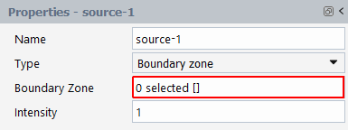
You can specify the inlet of the domain if the flow domain is open (entry and exit of fluid exist). Virtual particles will be randomly generated in the selected face zones.
Intensity identifies the relative number of points generated in the various sources. For example, if you define two sources with Intensity
1and3respectively, every pathline computed from source-1 will have three pathlines beginning from source-2.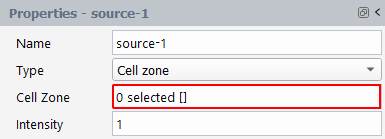
You can specify a part of the tracking zone (or the whole tracking zone) if the flow domain is closed (no entry and exit of fluid). The virtual particles will be randomly generated in the selected cell zones.
The Intensity identifies the relative number of points that are generated in the various sources. For example, if you define two sources with Intensity
1and3respectively, every pathline computed from source-1 will have three pathlines beginning from source-2.Imports a .csv (comma-separated values) file containing a list of initial positions of virtual particles.
The format of the .csv file may contain several sections. Each section contains the initial value of a given quantity for all material points. The first section must be for the
COORDINATES. The other sections may be used fortime,space_integration,direction_of_stretching,logarithm of stretchingandlabel.Important: Other names will not be recognized.
COORDINATES
 1; 0.1000000E+01; 0.0000000E+00; 0.0000000E+00;
 2; 0.2000000E+01; 0.0000000E+00; 0.0000000E+00;
 3; 0.3000000E+01; 0.0000000E+00; 0.0000000E+00;
 ..
10; 0.5000000E+01; 0.1000000E+00; 0.0000000E+00;

time
 1; 0.1000000E+01;
 2; 0.2000000E+01;
 3; 0.3000000E+01;
 ..
10; 0.1000000E+02;
Each section is separated by an empty line. The first line of each section contains the name of the quantity (upper case letters mandatory for COORDINATES, lower case for all other quantities). The following lines contain all numbers and reals separated by a semi-colon. These lines must end with a semi-colon. The first integer is the index of the material point, the other reals on the same line correspond to the initial value of the quantity component for that material point. COORDINATES and direction_of_stretching must have three components, while the other quantities only should have one component. The indexes must be identical throughout all sections.
Note: The Intensity property does not apply for CSV File sources, as you will compute the pathlines of all virtual particles defined in the .csv file.
Locate the initial position of the material points in a box overlapping (at least partially) the tracking domain.
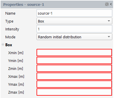
The box is defined by the coordinates of its two extreme corners:
Xmin [m], Ymin [m] and Zmin [m] for the lower-left-front corner.
Xmax [m], Ymax [m] and Zmax [m] for the upper-right-back corner.
There are two modes to generating the initial positions:
The initial positions of the material points are randomly generated in the box.
With this mode of generation, Intensity is required. The Intensity identifies the relative number of points that are generated in the various sources. For example, if you define two sources with Intensity
1and3respectively, every pathline computed from source-1 will have three pathlines beginning from source-2.
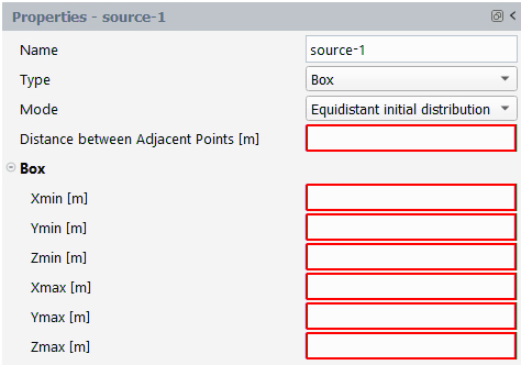
The material points, specified by you, are initially distributed at equal distance (
 ) between neighboring points. If the flow
domain is 2D, the points are distributed at vertex positions
of a lattice of identical equilateral triangles (see Figure 34.11: Equidistant Distribution of Points in a 2D
Box). If the flow domain is 3D, the points are distributed at
locations corresponding to the centers of close-packed equal
spheres. The generated points that are outside the flow
domain will be rejected.
) between neighboring points. If the flow
domain is 2D, the points are distributed at vertex positions
of a lattice of identical equilateral triangles (see Figure 34.11: Equidistant Distribution of Points in a 2D
Box). If the flow domain is 3D, the points are distributed at
locations corresponding to the centers of close-packed equal
spheres. The generated points that are outside the flow
domain will be rejected.

![]() Tracking
→ Quantities
Tracking
→ Quantities
A number of quantities can be evaluated along pathlines and are available in the Quantities panel.
Note: Quantities availabilities are dependent on a few conditions.
The current type of simulation opened (for example, the quantity is unavailable if your simulation is not thermal based).
The quantity not being previously evaluated as a derived quantity when computing the flow field.
Other quantities require another quantity to become available first (for example, requires and ).
Time and coordinates quantities are always saved.
You should only enable the quantities necessary for your study to save computation time and memory usage.
Space Integration
Enable to get the length of a trajectory up to the time
 .
.Rate of Stretching
Enable to get the rate of stretching
 (3D flow) or
  (2D flow). See Quantification of Mixing (Theoretical Background)
for more details.
(2D flow). See Quantification of Mixing (Theoretical Background)
for more details.Rate of Dissipation
Enable to get the rate of dissipation
 . It is the magnitude of the rate of deformation
tensor
. It is the magnitude of the rate of deformation
tensor  .
.See Quantification of Mixing (Theoretical Background) for more details.
Cumulated Dissipation
Enable to get the cumulated dissipation
 along the pathlines. This quantity is shown if the
quantity “rate of dissipation” is enabled.
along the pathlines. This quantity is shown if the
quantity “rate of dissipation” is enabled.Dc =

where
 is the time and
  is the rate of dissipation.
See Quantification of Mixing (Theoretical Background) for more details.
Direction of Stretching
Enable to get the direction of stretching n (3D flow) or m (2D flow) along the pathlines.
See Quantification of Mixing (Theoretical Background) for more details.
Logarithm of Stretching
Enable to get the logarithm of stretching
 (3D flow) or
  (2D flow) along the pathlines.
See Quantification of Mixing (Theoretical Background) for more details.
Instantaneous Efficiency of Stretching
Enable to get the instantaneous efficiency of stretching along the pathlines. It is defined as the ratio of the rate of stretching to the rate of dissipation. This quantity is available when and are enabled.
For 3D flows:
 =
= 
For 2D flows:
 =
= 
where
 is the rate of dissipation and
  or
or  are the rate of stretching in 3D or in 2D flows
respectively.
are the rate of stretching in 3D or in 2D flows
respectively.See Quantification of Mixing (Theoretical Background) for more details.
Time Averaged Efficiency of Stretching
For 3D flows: <
 > =
> = 
For 2D flows: <
 > =
> = 
where
 is the time,
  is the rate of dissipation,
  is the cumulated dissipation and
  ,
,  are the logarithm of stretching for 2d and 3D flow
respectively.
are the logarithm of stretching for 2d and 3D flow
respectively.See Quantification of Mixing (Theoretical Background) for more details.
Velocities
Enable to get the local velocity along the pathlines.
Pressure
Enable to get the local pressure along the pathlines.
Temperature
Enable to get the local temperature along the pathlines. This quantity is shown if the simulation is thermal based.
Shear Rate
Enable to get the local shear rate
 along the pathlines. This quantity is shown if
Rate of Dissipation is enabled. The local
shear rate can be defined as:
along the pathlines. This quantity is shown if
Rate of Dissipation is enabled. The local
shear rate can be defined as:where
 is the rate of dissipation and
  is the rate of deformation tensor.
Shear Viscosity
Enable to get the local shear viscosity along the pathlines. This quantity is available if the Viscosity derived quantity is enabled.
Stress Magnitude
Enable to get the local stress magnitude (stress in the direction of the velocity
 ) along the pathlines. This quantity is available
if the Stress derived quantity is
enabled.
) along the pathlines. This quantity is available
if the Stress derived quantity is
enabled.Mixing Index
Enable to get the local mixing index
 along the pathlines, It provides a local measure
of the dispersive mixing efficiency (see chapter 7 of [6]). This quantity is available when the
Mixing Index derived quantity is
enabled.
along the pathlines, It provides a local measure
of the dispersive mixing efficiency (see chapter 7 of [6]). This quantity is available when the
Mixing Index derived quantity is
enabled.The Mixing Index
 is defined as:
where
 is the shear rate and
  is the magnitude of the vorticity vector. The
mixing index
is the magnitude of the vorticity vector. The
mixing index  indicates, locally, whether the flow is rigid (Mi
= 0), a shear flow (Mi = 0.5), or an extensional flow (Mi =
1).
indicates, locally, whether the flow is rigid (Mi
= 0), a shear flow (Mi = 0.5), or an extensional flow (Mi =
1).Melting Index
Enable to get the local melting index
 along the pathlines. This quantity is shown if the
quantities Temperature and Shear
Viscosity are enabled.
along the pathlines. This quantity is shown if the
quantities Temperature and Shear
Viscosity are enabled.The Melting Index, (used in [3] to characterize the quality of the glass melting in a furnace), is defined as:
where
 is the time,
  is the shear viscosity and
  is the temperature.
Determinant of Tensor F (det F)
Enable to measure the accuracy of the computation. As flow is incompressible, it should remain equal to 1 along any pathline.
Divergence of Velocities (div V)
Enable to measure the accuracy of the computation. As flow is incompressible, it should remain equal to 0 along any pathline.


![]() Tracking
→ Controls
Tracking
→ Controls
In the Controls panel, you can define the parameters necessary to initialize the kinematic quantities, provide some characteristics of the flow field, evaluate accurately the pathlines and specify the mode of storage of the trajectories.
Lifetime [s]
Allows you to specify the lifetime of each virtual particle. Once this value is reached, Fluent Materials Processing stops to evaluate the pathline of the current virtual particle.
Velocity Magnitude [m/s]
Specify the typical velocity magnitude of the particles. The average velocity magnitude of the flow field can be provided.
Flow Regime
This option is available for transient flows only. You specify whether the flow is continuous transient or piecewise steady.
Start Id
This option is available for transient flows only. For tracking tasks, it is assumed that the flow is periodic. You must specify which time step will be the first to be used for the pathlines evaluation (first, last, or intermediate). During pathline evaluations, you use the flow fields of each time step in a loop until the lifetime of the particles is reached.
Intermediate Step
This option is only available for transient flows and when Start Id has been set to . Specify the initial step used for pathline evaluations.
Constraint on Tensor F
This option is available for 2D flows only. By enabling this option, you normalize the tensor F regularly during the pathline evaluation allowing its determinant to remain equal to 1.
Initial Stretching Direction
This option is used for stretching quantities. An initial vector must be specified for each virtual particle. For example, random (different for each virtual particle) or imposed (same for all virtual particles). When the virtual particle travels within the flow, the vector will reorient and stretch.
Imposed Direction
Dx, Dy, Dz
When specifying Initial Stretching Direction, you can specify the X, Y, Z components of the vector N (if flow is 3D) or M (if flow is 2D).
Storage Controls
Storage Mode
Various modes of storage are available to store virtual particle positions such as , , , , .
Note: In regards to memory consumption, consumes the most. When the flow field is transient, , are preferred. While for steady flows with an inlet/outlet, , are preferred.
Time Step [s]
Specify the time step before storing the position of a virtual particle.
Displacement [m]
Specify the displacement before storing the position of a virtual particle.
Maximum Number of Files
Specify the number of files that will contain pathlines. It is preferable to have multiple, smaller sized files rather than a large one.
Maximum Number of Pathlines per File
Specify the maximum number of pathlines that will be saved in a single file.
Maximum CPU Time per File [hour]
Specify the CPU time needed to generate a file. As soon as the specified CPU time is reached, the current file is closed and another is created to contain the next pathlines.
Save in Polyflow MIX Files
Enable to generate Ansys Polyflow *.mix files containing the pathlines (*.mix files are mandatory to perform statistical analysis).
Save in CFD-Post TRK Files
Enable to generate CFD-Post *.trk files containing the pathlines.
Save in Fieldview FVP Files
Enable to generate Fieldview *.fvp files containing the pathlines.
Advanced Controls
Relative Tolerance on a Distance
This option is an advanced parameter used to evaluate the pathlines. A point is considered on the border of a finite element if its distance (in the parent element) to the border is less than this tolerance.
Relative Tolerance on a Velocity
This option is an advanced parameter used to evaluate the pathlines. A point is considered as a stagnation point if its velocity (in the parent element) is less than this tolerance.
Relative Tolerance on a Time
This option is an advanced parameter used to evaluate the pathlines. A time step is considered as negligeable if it is less than this tolerance. It will be used to stop the iterative Newton-Raphson procedure that finds the time step needed to reach the border of the current finite element containing the point.
Number of Steps per Cell
This option is an advanced parameter used to evaluate the pathlines. You indicate how many Runge-Kutta steps a particle will cross each finite element. The initial time step of integration for each element is determined by the following formula.
Initial time step in element E = Size(E) / velocity magnitude / number of steps per cell
Keywords
Advanced option for the solver and should not be used unless recommended by Ansys Customer Support.


Once all Tracking parameters are defined, you can
launch your calculation using ![]() Tracking
→ Run Calculation
Tracking
→ Run Calculation
The following are available to you within the Properties - Run Calculation panel:
Verify and ensure the setup of your tracking simulation is valid. Any relevant messages are displayed in the Console window notifying you of any discrepancies.
Once your setup is valid, click to start the solver.
Pauses the solver once the calculation has started.
Interrupts the solver once the calculation has started.
Restarts the solver and completes the interrupted calculation.
Allows you to view instructions about the solution transcript once the calculation completes. It is available as a docked tab next to the Graphics window.
It allows to start CFD-Post in order to see the pathlines saved (if asked by the user) in *trk files.
Polyflow .mix files can be loaded into Polystat for
visualization and statistical analysis. To launch Polystat from Fluent Materials Processing,
select Tracking → Run
Calculation![]() Polystat
Polystat
The .mix files can be found in the Tracking directory under the project directory.
CFD-Post .trk files can be loaded into CFD-Post for
visualization. To launch CFD-Post from Fluent Materials Processing, select
Tracking → Run
Calculation![]() CFD-Post.
CFD-Post.
The .trk files can be found in the Tracking directory under the project directory.
The Fieldview .fvp files can be loaded into Fieldview for visualization. Fieldview can only be launched outside of Fluent Materials Processing. The .fvp files can be found in the Tracking directory under the project directory.
This section describes the following topics:
After the calculation of a large set of pathlines (performed previously in the Tracking tab), it is now possible to treat those results to obtain a global and objective overview of the mixing process (but not only) in the current flow. To achieve this goal, one performs a statistical treatment on the pathlines. We consider here two kinds of flow: steady state flows with inlet and outlet sections (flow in an open domain) or transient flows in a closed domain (with or without moving parts). We are interested to analyse the evolution of some properties during the process: as a function of “space”, for open domains, from the inlet to the outlet, or as a function of time for closed domains. We define thus a slicing on the pathlines (a set of cutting planes for open domains, and a set of times for closed domains): for each slice, we get thus a sampling of values on which we can perform some statistical treatment. With such a method, e.g., we can analyse how stretching evolves in a kenics mixer or in a batch mixer. We can also analyse the distribution of materials points initially concentrated in a small box.
To achieve this goal, one performs a statistical treatment on the pathlines. This is done in several steps.
Under the Pathlines Sets node, you can specify the pathlines that will be used for the statistical task: they are provided by the Tracking task, or by loading mixing files coming from another project. Moreover, you can create “derived” pathlines sets based on these primary sets: by filtering them, or through Boolean operations applied on them. For example, you can eliminate all the trajectories that terminated abnormally (for example, on a wall). Moreover, specific kinds of pathlines sets are also provided: it is possible to extract a single pathline from a set, or to detect stagnation points.
Under the Quantities node, as soon as you have uploaded pathlines, a set of quantities will become visible. You can ask to calculate new quantities evolving along the trajectories. For example, you can define any concentration field, extract a component of a vectorial quantity, or ask for the magnitude of a quantity. These new quantities are always a combination of existing quantities (those calculated previously and stored in the mixing result files).
Under the Slicing node, you determine the way to slice the selected trajectories. For example, suppose you are analyzing the flow through a cylinder, like the one shown in the following picture:
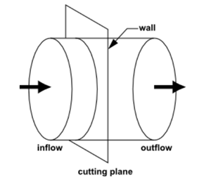
To analyze this flow, locate a set of material points in the inflow
section, and calculate their trajectory until they reach the outflow section.
You will then cut the pathlines with planes disposed regularly from the entry to
the exit (this is the slicing step). In each plane, you will calculate
statistical functions. Those functions will evolve from entry to exit and show
the way the mixing changes (among other characteristics, because one can perform
statistics on any quantities as soon as they are known along the pathlines. E.G.
residence time, temperature, shear rate, ..). Note: If the flow occurs in a
closed domain, you want to know the time evolution of statistical functions and
the slicing will be done on the time.
Under the Functions node, you define the set of statistical functions that you want to calculate on the defined set of slices. E.G. probability, density of probability, histograms, .. on quantities. But one can also define more specific functions to evaluate the distribution mixing.
Under the Run Calculation node, you will be able to calculate effectively the defined pathlines sets, slicings and functions. This calculation can take a while to complete. A summary is provided to check the solver actions.
Under the Charts node, you will be able to define charts to visualize your statistical functions.
Eventually, it is also possible to export pathlines sets, slicings and functions to visualize them in CFD-Post, Fieldview, Polystat and Excel. NB. Only Polystat allows you to visualize easily pathlines in transient flows involving moving parts.
Two properties may affect the pathlines and statistics calculations:
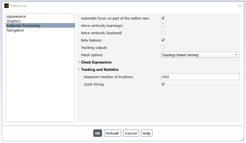
Maximum number of positions: the computation of a single pathline may involve many intermediate positions from the starting point until it reaches the exit and/or its lifetime. In general, it is not necessary to store all these positions for further statistical analysis. With this property, you limit the number of stored positions. By this way, we also reduce the size of the mixing files and accelerate the statistics computation.
Quick Slicing: when performing a space slicing, a pathline may cross several times the same slice (E.G., when backflow is present). By enabling this property, we search only for the first intersection between the pathline and the slice. By this way, we accelerate the statistics computation and avoid some statistical bias (a single material point counted several times).
When we do statistics on a population of material points, two important points must be kept in mind:
the population of material points must be large enough to get accurate and objective statistics. Especially if one wants to compare different setups and/or geometries.
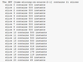
as we calculate statistical functions on a set of slices, it is important to remember that each slice should contain (almost) same number of instants. If the number of instants decreases too much, the statistics will be biased. We can check that number in the transcript window (click on “View Listing” in the Run Calculation panel): in the following example, we see that the number of instants diminishes dramatically after slice #14, leading to unusable statistics.
In order to facilitate definition of a statistical analysis based on set of pathlines evaluated earlier in the tracking task (of the same project), a few templates are available:
Kinematic analysis vs time
Kinematic analysis vs space
Distribution analysis vs time
Distribution analysis vs space
These templates can be found in the ribbon, on the Statistics page:

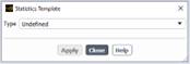
Click on “Use Template..”: a popup-menu appears where you can select the template type:
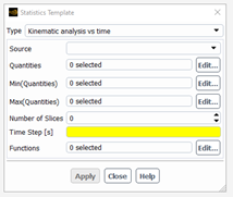
For the Kinematic analysis vs time, we assume that the flow occurs in a closed domain (no inlet, no outlet) and changes with time (e.g. in a batch mixer). We are interested here to analyse how the stretching of small pieces of matter attached to the material points and/or other quantities evaluated along the pathlines in the tracking task (e.g. temperature, shear stress, mixing index, ..) change with time. The user will have to specify the source of the material points (defined in the tracking task), a few parameters to define the slicing along the time (number of slices, time step – we assume the time starts at t=0 s), select the quantities (including the minimum and the maximum of some quantities) he wants to summarize in a few statistical functions, and eventually, choose the statistics to perform.
When all the properties of the panel are defined, click on “Apply” : the panel closes and the Fluent Materials Processing App will generate all the relevant objects (pathlines sets, quantities, slicings and functions) and populate the Statistics sub-tree in the Outline View. Once this is done, the user can modify or fill some missing properties. Eventually, he can check the setup and start the calculation, by clicking on “Check” or “Calculate” buttons respectively in the ribbon (in the Statistics page). After the calculation, the user will have to define a few charts to visualize his results.
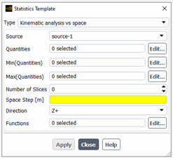
For the Kinematic analysis vs space, we assume that the flow occurs in an open domain (with inlet and outlet) and is steady state (e.g. in a Kenics mixer). We are interested here to analyse how the stretching of small pieces of matter attached to the material points and/or other quantities evaluated along the pathlines in the tracking task (e.g. temperature, shear stress, mixing index, ..) evolve from the inlet to the outlet of the flow domain. To do so, we have to define a set of cutting planes starting at inlet and located at regular space step in the flow direction (supposed to be aligned with one axis). The user will have to specify the source of the material points (defined in the tracking task), a few parameters to define the slicing in space (number of slices, space step, direction of slicing (X+, Y+, Z+, X-, Y- and Z-), select the quantities (including the minimum and the maximum of some quantities) he wants to summarize in a few statistical functions, and eventually, choose the statistics to perform.
When all the properties of the panel are defined, click on “Apply” : the panel closes and the Fluent Materials Processing App will generate all the relevant objects (pathlines sets, quantities, slicings and functions) and populate the Statistics sub-tree in the Outline View. Once this is done, the user can modify or fill some missing properties: it is important here to check the parameters of the slicing, specially, the initial slice position and the normal direction to the slices. Eventually, he can check the setup and start the calculation, by clicking on “Check” or “Calculate” buttons respectively in the ribbon (in the Statistics page). After the calculation, the user will have to define a few charts to visualize his results.
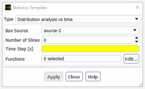
For the Distribution analysis vs time, we assume that the flow occurs in a closed domain (no inlet, no outlet) and changes with time (e.g. in a batch mixer). We are interested here to analyse how the material points initially concentrated in a box will spread and fulfill the whole flow domain. In the tracking task, two sources must have been defined: one box and the whole flow domain. The user will have to specify the box source of the material points, a few parameters to define the slicing along the time (number of slices, time step – we assume the time starts at t=0 s), and choose the statistics to perform: 3 functions are available (distance distribution, distribution in zones and axial distribution), each one requiring to define some properties:
Distance distribution: maximum distance (see the paragraph on “distance distribution function” for further details)
Distribution in zones: zone size (see the paragraph on “distribution in zones” for further details). The number of zones in each direction will be evaluated assuming the size of the smallest box surrounding the whole mesh:
Number of zones along X = round[abs(xmax-xmin)/zone_size]
Number of zones along Y = round[abs(ymax-ymin)/zone_size]
Number of zones along Z = round[abs(zmax-zmin)/zone_size]
Axial distribution: axis (X, Y, Z)
In this case, we define a new quantity (of “extract” type) based on the component of the coordinates selected as the axis. We will see how the values of this component spread with time (for the set starting from the box), and how this distribution matches the perfect distribution (corresponding to the set defined on the whole flow domain).
When all the properties of the panel are defined, click on “Apply” : the panel closes and the Fluent Materials Processing App will generate all the relevant objects (pathlines sets, quantities, slicings and functions) and populate the Statistics sub-tree in the Outline View. Once this is done, the user can modify or fill some missing properties. Eventually, he can check the setup and start the calculation, by clicking on “Check” or “Calculate” buttons respectively in the ribbon (in the Statistics page). After the calculation, the user will have to define a few charts to visualize his results.
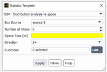
For the Distribution analysis vs space, we assume that the flow occurs in an open domain (with inlet and outlet) and is steady state (e.g. in a Kenics mixer). We are interested here to analyse how the material points initially concentrated in a box located in the inlet will spread and fulfill the flow domain and especially the outlet section. To do so, we have to define a set of cutting planes starting at inlet and located at regular space step in the flow direction (supposed to be aligned with one axis). Previously, in the tracking task, two sources must have been defined: one box located in the inlet and the inlet. The user will have to specify the box source of the material points (defined in the tracking task), a few parameters to define the slicing in space (number of slices, space step, direction of slicing (X+, Y+, Z+, X-, Y- and Z-), and choose the statistics to perform: 2 functions are available (distance distribution and distribution in zones), each one requiring to define some properties:
Distance distribution: maximum distance (see the paragraph on “distance distribution function” for further details)
Distribution in zones: zone size (see the paragraph on “distribution in zones” for further details). The number of zones in each direction (other than the flow direction) will be evaluating assuming the size of the smallest box surrounding the whole mesh:
Number of zones along X = round[abs(xmax-xmin)/zone_size]; (reset to 1 if flow direction is X+ or X-)
Number of zones along Y = round[abs(ymax-ymin)/zone_size]; (reset to 1 if flow direction is Y+ or Y-)
Number of zones along Z = round[abs(zmax-zmin)/zone_size]; (reset to 1 if flow direction is Z+ or Z-)
When all the properties of the panel are defined, click on “Apply” : the panel closes and the Fluent Materials Processing App will generate all the relevant objects (pathlines sets, quantities, slicings and functions) and populate the Statistics sub-tree in the Outline View. Once this is done, the user can modify or fill some missing properties: it is important here to check the parameters of the slicing, specially, the initial slice position and the normal direction to the slices. Eventually, he can check the setup and start the calculation, by clicking on “Check” or “Calculate” buttons respectively in the ribbon (in the Statistics page). After the calculation, the user will have to define a few charts to visualize his results.
We specify here the different pathlines on which we will perform a statistical analysis. There are several types of pathlines sets, but one need at least one set of the “From tracking task” type or of the “From mixing files” type.
To create them, go in the "Statistics" properties panel:
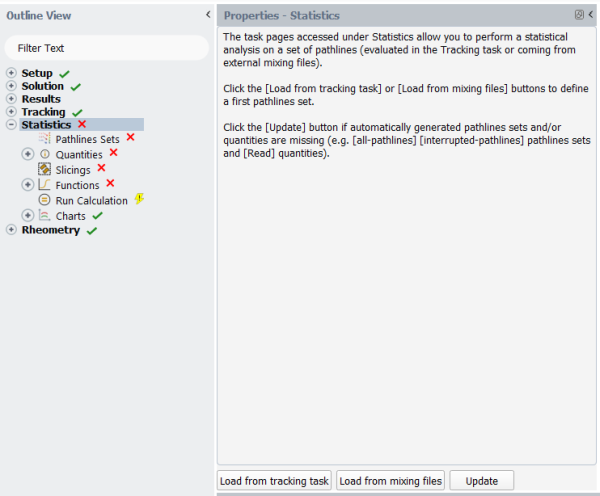
and click on the "Load from tracking task" or "Load from mixing files" buttons to create the corresponding sets and load the mixing files (a specific "Load" button must be clicked in these sets to perform effectively the loading - this is not automatic).
After the load, some new pathlines sets are created together with a list of quantities. See below for further details.
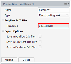
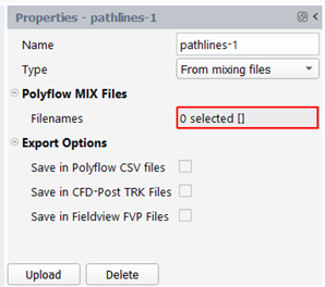
Once the type is selected, new properties become visible:
For "From tracking task" type: one has to load the mixing files computed in the tracking task (meaning that this part of the project must be up-to-date). To do so, click on the "Load" button at bottom of the property panel. After the loading, the Filenames property should be completed, and some new pathlines sets (all pathlines, interrupted pathlines) and quantities (the quantities asked for in the tracking task) should appear in the Outline View.
For “From mixing files” type: one has to load the mixing files computed in another project. To do so, click on the “Load” button at bottom of the property panel. One has to specify in a browser the mixing files to be loaded. After the loading, the Filenames property should be completed, and some new pathlines sets (all pathlines, interrupted pathlines) and quantities (the quantities asked for in the tracking task) should appear in the Outline View.
For “All pathlines” and “Interrupted pathlines”, no additional property is available. These two sets are automatically created after an “Load” action (see the two previous paragraphs).
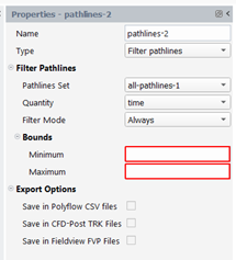
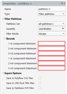
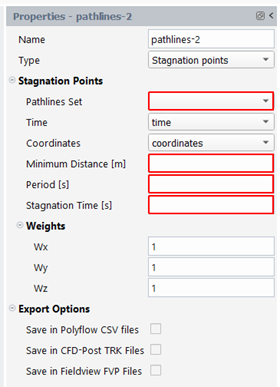
For “Filter pathlines” type, we will select a sub-set of pathlines, from another one, that respects some condition. The following properties must be specified:
Pathlines Set: enter the pathlines set on which the filtering will be applied.
Quantity: enter the quantity to be used to define the condition
Filter Mode: “Always”, “One time (at least)”, “Never”
Bounds: if the quantity is a scalar, a minimum and a maximum must be provided. If the quantity is a vector, a range for each component of the vector.
If one uses the “Always” filter mode, we keep a pathline if the selected quantity is always in the specified bounds.
If one uses the “One time (at least)” filter mode, we keep a pathline if the selected quantity is for a single position (at least) in the specified bounds.
If one uses the “Never” filter mode, we keep a pathline if the selected quantity is always out of the specified bounds.
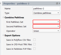
For “Combine pathlines” type, we will perform some boolean operation between two pathlines sets. Four operators are available:
Union: the new set will contain the pathlines of both sets (A+B+C in picture below)
Intersection: the new set will contain the pathlines that belong to the two sets (C in picture below)
Minus: the new set will contain the pathlines of the first set that do NOT belong to the second set (A in picture below)
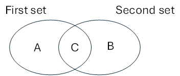
Difference: the new set will contain the pathlines that belong to each set but do not belong to the other set (A+B in picture below)
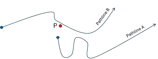
For “Single pathline” type, we will select one pathline from a set that respects some condition. The following properties must be specified:
Pathlines Set: enter the pathlines set on which the search will be applied.
Coordinates: enter the coordinates quantity to be used to define the condition
Closest Mode: “Initially”, “At any moment”
Point: provide here a position
If one uses the “Initially” closest mode, we keep the pathline whose starting position is the closest to the specified point. (Pathline A in the figure below)
If one uses the “At any moment” closest mode, we keep the pathline whose the distance is the minimum to the specified point. (Pathline B in the figure below)
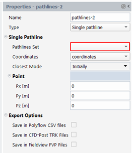
For “Stagnation points” type, we want to determine if some stagnation points exist among a pathlines set. Two kinds of stagnation points may be searched: the one close to a fixed wall, the one that are close to a rotating wall (moving part), and that have a circular path.
The following properties must be specified:
Pathlines Set: enter the pathlines set on which the search will be applied.
Time and Coordinates quantities
Minimum Distance: a point is stagnant if the distance between its initial position and some of its successive positions are less than this minimum distance.
Period P:
To detect stagnation points close to a fixed wall, the period P may take any value. However, if you want to detect stagnation points close to a rotating wall (of a moving part, for example), you have to specify the period P of rotation of the moving part.
Only the positions
 , for time
  , corresponding to a multiple of P will be
tested, from 0 until stagnation time. For example,
, corresponding to a multiple of P will be
tested, from 0 until stagnation time. For example,  will be tested at times
  stagnation time
Stagnation time: must be less than the residence time
Weight
 : it is a way to weight specifically some
components of the coordinates when computing distance
between
: it is a way to weight specifically some
components of the coordinates when computing distance
between  and
and  :
: 
By default, the weights are set to 1
The Export Options are always available: with these properties, one can export pathlines sets for further analysis in other tools. Enable the outputs of interest:
Save in Polyflow CSV files: csv files are generated for analysis in Excel.
Save in CFD-Post TRK files: trk files are generated for visualization in CFD-Post.
Save in Fieldview FVP files: fvp files are generated for visualization in Fieldview.
All the files will be stored in the Statistics/Outputs directory under the project directory.
We specify here the quantities of interest for further statistical analysis: among of them, some quantities are automatically created after the definition of pathlines sets (of type: “from tracking task” and “from mixing files”). These quantities cannot be modified. Moreover, the user can define new quantities, based on “Read” quantities but also on the ones the user has created: by this way, it can define complex quantities relevant for his process. Be careful not to define circular dependencies between quantities. Note that if you save the pathlines sets by using the Export Options (see above for further details), the new quantities will be also available for visualization (in Polystat, CFD-Post or Fieldview, depending on the saving options that were enabled).
We will now examine them.
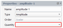
Amplitude
We create a quantity that is the absolute value of a scalar quantity or the magnitude of a vector quantity. The result quantity is a scalar. Select “Amplitude” for the Type and select the input quantity in the drop-down list “Quantity” in the property panel:
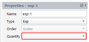
Exponential
We create a quantity that is the exponential of a scalar quantity. The result quantity is a scalar. Select “Exp” for the Type and select the input quantity in the drop-down list “Quantity” in the property panel:
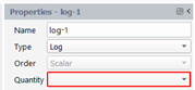
Logarithm
We create a quantity that is the natural logarithm of a scalar quantity. The result quantity is a scalar. Select “Log” for the Type and select the input quantity in the drop-down list “Quantity” in the property panel:
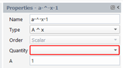
A ^ x
We create a quantity that is the exponent of a positive constant A by a scalar quantity. The result quantity is a scalar. In the property panel, select “A^x” for the Type, select the input quantity in the drop-down list “Quantity” and define the positive constant A:
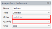
Time Derivation
We create a quantity that is the time derivation of another quantity. The result quantity can be a scalar or a vector, depending on the order of the input quantity. The accuracy of this quantity is dependent on the number of instants stored along each pathline: few instants will lead to poor evaluation of the derivate. In the property panel, select “Derivate” for the Type, select the input quantity in the drop-down list “Quantity” and select the time quantity:
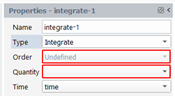
Time Integration
We create a quantity that is the time integration of another quantity. The result quantity can be a scalar or a vector, depending on the order of the input quantity. The accuracy of this quantity is dependent on the number of instants stored along each pathline: few instants will lead to poor evaluation of the integral. In the property panel, select “Integrate” for the Type, select the input quantity in the drop-down list “Quantity” and select the time quantity:
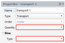
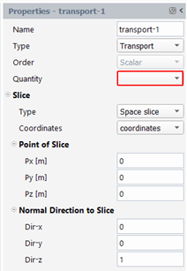
Transport
With this type of quantity, we will transport the value of a quantity along the whole pathline, the value being taken in a given slice (see figure below). The result quantity can be a scalar or a vector, depending on the order of the input quantity. Two kinds of slices may be defined: a slice on time (a time value and the time quantity must be specified) or a slice on space (a point and a normal to the cutting plane and the coordinates quantity must be specified).
In the property panel, select “Transport” for the Type, select the input quantity in the drop-down list “Quantity” and select the slice type:
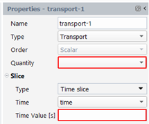
If you selected a time slice, the property panel allows you to enter a time value and the time quantity, as shown below:
If you selected a space slice, the property panel allows you to enter a point of the slice, the normal direction to the slice and the coordinates quantity, as shown below:
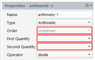
Arithmetic operations
We create a quantity that is the result of an arithmetic operation (addition, subtraction, multiplication, and division) between two quantities. The result quantity can be a scalar or a vector, depending on the order of the two quantities. Some combination of input quantities is not allowed depending on the selected operator: with the sum and subtraction, both quantities must have same order, with multiplication and division, the first quantity may be a scalar or a vector, but the second quantity must be a scalar. In the property panel, select “Arithmetic” for the Type, select the two quantities in the drop-down list “First Quantity” and “Second Quantity” respectively and select the operator:
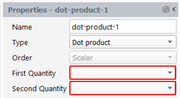
Dot Product
We create a quantity that is the dot product between two vector quantities. The result quantity is a scalar. In the property panel, select “Dot product” for the Type, select the two quantities in the drop-down list “First Quantity” and “Second Quantity” respectively:
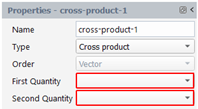
Cross Product
We create a quantity that is the cross product between two vector quantities. The result quantity is a vector. In the property panel, select “Cross product” for the Type, select the two quantities in the drop-down list “First Quantity” and “Second Quantity” respectively:
Extract
We create a quantity that is the i-th component of a vector quantity. The result quantity is a scalar. In the property panel, select “Extract” for the Type, select the input quantity in the drop-down list “Quantity” and select the component (1, 2 or 3):
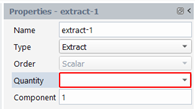
For example, if the coordinates (x,y,z) is the selected quantity and the 2-nd component is chosen, then the extracted component will be y and it will be stored in the new quantity.
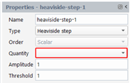
Heaviside step
We create a step quantity that is based on a scalar quantity. The result quantity is a scalar. For each instant of a pathline, we compare the local value V of the input quantity to a threshold value T: if V is greater than T, then the local value of the new quantity will be a given amplitude A, otherwise the local value of the new quantity will be zero. In the property panel, select “Heaviside step” for the Type, select the input quantity in the drop-down list “Quantity” and define the threshold and the amplitude:
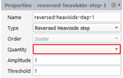
Reversed Heaviside step
We create a reversed step quantity that is based on a scalar quantity. The result quantity is a scalar. For each instant of a pathline, we compare the local value V of the input quantity to a threshold value T: if V is lower than T, then the local value of the new quantity will be a given amplitude A, otherwise the local value of the new quantity will be zero. In the property panel, select “Reversed Heaviside step” for the Type, select the input quantity in the drop-down list “Quantity” and define the threshold and the amplitude:
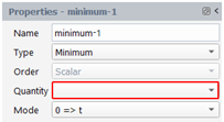
Minimum
We create a quantity that is based on a scalar quantity. The result quantity is a scalar. There are two modes for defining the minimum:
Mode "
 ": for each instant of a pathline, we
compare the local value V of the input quantity to all
previous values: the new value at that instant will be the
minimum obtained:
": for each instant of a pathline, we
compare the local value V of the input quantity to all
previous values: the new value at that instant will be the
minimum obtained: 
Mode "
 ": for a pathline, we search the minimum of
the local value V of the input quantity among all instants:
the new value for all instants will be that minimum:
": for a pathline, we search the minimum of
the local value V of the input quantity among all instants:
the new value for all instants will be that minimum: 
In the property panel, select “Minimum” for the Type, select the input quantity in the drop-down list “Quantity” and select the mode:
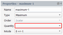
Maximum
We create a quantity that is based on a scalar quantity. The result quantity is a scalar. There are two modes for defining the maximum:
Mode "
 ": for each instant of a pathline, we
compare the local value V of the input quantity to all
previous values: the new value at that instant will be the
maximum obtained:
": for each instant of a pathline, we
compare the local value V of the input quantity to all
previous values: the new value at that instant will be the
maximum obtained: 
Mode "
 " : for a pathline, we search the maximum
of the local value V of the input quantity among all
instants: the new value for all instants will be that
maximum:
" : for a pathline, we search the maximum
of the local value V of the input quantity among all
instants: the new value for all instants will be that
maximum:
In the property panel, select “Maximum” for the Type, select the input quantity in the drop-down list “Quantity” and select the mode:
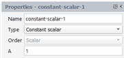
Constant Scalar
We create a quantity that is a scalar quantity. For each pathline, the local value of this new quantity will be the same for all instants. In the property panel, select “Constant scalar” for the Type, and define a constant value A:
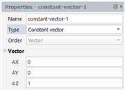
Constant vector
We create a quantity that is a vector quantity. For each pathline, the local vector of this new quantity will be the same for all instants. In the property panel, select “Constant vector” for the Type, and define the three components of the Vector (AX, AY, AZ):
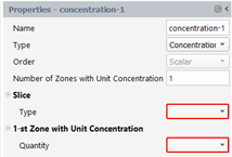
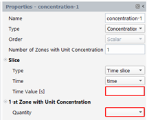
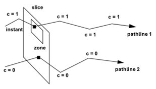
Concentration
With this type of quantity, we will transport a concentration value (0 or 1) along the whole pathline, the value being defined in a given slice (see figure below): the user specifies zones (for each zone, a quantity and bounds must be provided: if the value of the quantity in the slice is ranged in the bounds, then the local concentration will be one; if the instant i is out of the bounds of all zones, then the concentration will be zero). The user can define up to 5 zones. The result quantity is a scalar. Two kinds of slices may be defined: a slice on time (a time value and the time quantity must be specified) or a slice on space (a point and a normal to the cutting plane and the coordinates quantity must be specified).
Note that the concentration field is constant for a material point (no diffusion, no chemical reactions), the value of the concentration is transported along the trajectories without changing.
In the property panel, select “Concentration” for the Type, enter the number of zones and select the slice type:
If you selected a time slice, the property panel allows you to enter a time value and the time quantity, as shown below:
If you selected a space slice, the property panel allows you to enter a point of the slice, the normal direction to the slice and the coordinates quantity, as shown below:
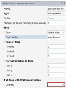
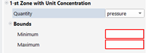
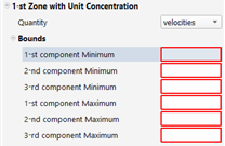
Next, for each zone, specify the quantity and the bounds of the filter, as shown below:
We specify here at which time or space interval we will cut the pathlines. Statistical functions will be later applied on each of those slices.
The list of available slicing types:

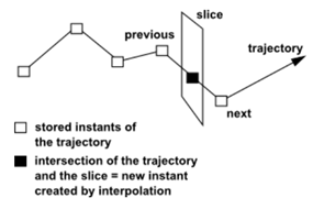
Remember that a pathline is a set of instants ordered in time. Each slice will contain a set of instants that are the intersections of the slice and the pathlines. If the intersection of a pathline and a slice is not a stored instant, a new instant is created by interpolation with the previous and the next instants that surround the intersection, as shown below:
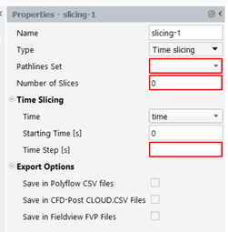
Time Slicing: with this kind of slicing, we cut the trajectories at regular time intervals. This kind of slicing should be used for flow fields in closed domain (e.g. batch mixers), where the process is time dependent. The user has to specify a pathlines set, a number of slices, a time quantity, a starting time ts and a time step dt.
The slices will be done at times: ts, ts+dt, ts+2dt, ..
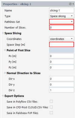
Space Slicing: with this kind of slicing, we cut the trajectories with planes at regular space intervals in a given direction. This kind of slicing should be used for flow fields in open domain (e.g. static mixers), where the process is steady state. The user has to specify a pathlines set, a number of slices, a coordinates quantity, a space step dl, a starting point ps and a normal direction to the slices N.
The successive planes contain point: ps, ps+dl * N, ps+2dl*N, .. and have normal N
Manual Slicing: with this kind of slicing, the user defines each slice one by one. By this way, slices are defined at precise location (in space or time), when it is not useful to get them at regular intervals. The user has to specify first a pathlines set and a number of slices n. When that number is specified a set of slices is visible in the property panel:
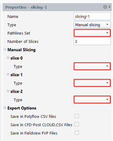
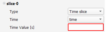
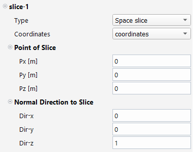
For each slice, the user will have to specify its type (Time slice or Space slice) and enter specific properties: a time quantity and a time value, if this is a time slice. While for a space slice, we need a coordinates quantity, a position of the cutting plane and a normal direction to the plane.
This kind of slicing is useful when the number of slices is small. Otherwise, it is rapidly cumbersome to enter numerous properties in a long panel.
The Export Options are always available: with these properties, one can export the set of slices for further analysis in other tools. Enable the outputs of interest:
Save in Polyflow CSV files: csv files are generated for analysis in Excel.
Save in CFD-Post CLOUD.CSV files: cloud.csv files are generated for visualization in CFD-Post.
Save in Fieldview FVP files: fvp files are generated for visualization in Fieldview.
All the files will be stored in the Statistics/Outputs directory under the project directory.
There are three kinds of functions available:
functions based on a pathlines set or a single pathline
functions based directly on the instants of slices
functions based on other functions
Different types are possible:
Quantity along a pathline :
The user has to specify a single pathline, a quantity to visualize and a time quantity.
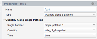
The corresponding chart will present the time evolution of the given quantity for that pathline:
Sum
To calculate the sum function of a quantity, you need to specify which slicing to be used and to select a quantity. When the slicing type is a space slicing, the weight mode and a velocities quantity must be provided. Additional information on weighting is available in the annexes (§ on Weighting).
For each slice, we sum the value of the quantity of all the instants in the slice.
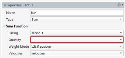
The corresponding chart will present the evolution of the sum of a quantity along the slices : the X axis is the slice index, and the Y axis is the quantity.
Mean and Standard Deviation
To calculate the mean and standard deviation functions of a quantity, you need to specify which slicing to be used and to select a quantity. When the slicing type is a space slicing, the weight mode and a velocities quantity must be provided. Additional information on weighting is available in the annexes (§ on Weighting).
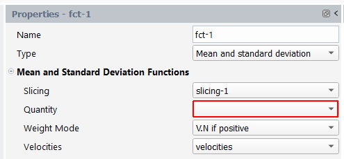
The corresponding chart will present two curves: the evolution along the slices of the mean and of the standard deviation of a quantity : the X axis is the slice index, and the Y axis is the quantity .
Correlation Function
To analyze a possible correlation between two quantities in two slices of the same slicing: select a slicing, and for that slicing, specify two slice indices and quantities.
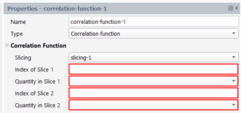
The corresponding chart will present on the X axis the quantity associated with the first slice, and on the Y axis the quantity associated with the second slice. Each dot of the plot corresponds to a pair { Quantity1(slice1); Quantity2(slice2) } of a virtual particle.
Note that the line type must be modified in the Plots page and set to “Point – Circle” (Dataset, … / Plot settings / set curve type).
Probability function
To calculate the evolution of the probability function of a quantity, you need to specify a slicing, a quantity and the number of values to represent the curves (one evaluates one curve per slice). When the slicing type is a space slicing, the weight mode and a velocities quantity must be provided. Additional information on weighting is available in the annexes (§ on Weighting).
For a given slice, the probability is always ranged from 0 (for the minimum value of the quantity in the slice) to 1 (for the maximum value of the quantity in the slice).
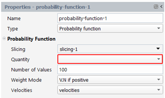
If you visualize this function for a given slice, the quantity is on the X axis and the probability on the Y axis.
Density of Probability Function
To calculate the evolution of the density of probability function of a quantity, you need to specify a probability function (defined before) and the number of values to represent the curves (one evaluates one curve per slice): that number of values should be less than the number of values used to represent the probability function, in order to avoid too many wiggles: a good practice is to use half the number of values that represent the probability functions. If they persist, a smoothing on the density curves can be performed (see here after).

There is a list of probability functions P (one for each slice of a sorted list) and you obtain a density of probability function f for each slice S:
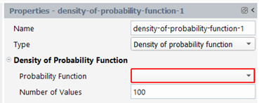
If you visualize this function for a given slice, the quantity is on the X axis and the density of probability on the Y axis.
Percentiles
To calculate the evolution of percentiles of a quantity along slices, you need to specify a probability function (defined before) and a list of values (ranged from 0 to 100 %).
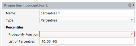
The corresponding chart will present a curve for each percentile: the evolution along the slices of the x-th percentile of a quantity : the X axis is the slice index, and the Y axis is the quantity ..
How to interpret such curves? For a given slice S, draw mentally a vertical line: that line will cut your percentiles (1Oth, 50th, 90th). Let note P10(S), P50(S) P90(S) the corresponding values obtained. The value of P10(S) indicates that in slice S, 10% of the instants have a value lower than P10(S) and 90% have a value higher than that value. The value of P50(S) indicates that in slice S, half the instants have a value lower than P50(S) and half have a value higher than that value. The value of P90(S) indicates that in slice S, 90% of the instants have a value lower than P90(S) and 10% have a value higher than that value.
So, in conclusion, P50 provide a similar information than the mean (but is not identical!!), and the distance between P10 and P90 provide similar information than the standard deviation (but is not identical!!).
Histograms
To calculate the evolution of histograms of a quantity along slices, you need to specify a probability function (defined before) and a list of values to define the intervals of the histograms (ranged from the absolute minimum and absolute maximum of the quantity selected in the parent probability function.
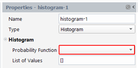
From the list of probability functions (one for each slice of a sorted list), you obtain a histogram function for each slice. If you visualize this function for a given slice, the specified intervals of values (you chose the corresponding quantity when you defined the probability function) are on the X axis and the percentage of instants of the slice having a quantity value in each interval is on the Y axis.
Smoothing Function
To create a smoothing function, you have to select the function to smooth and the type of smoothing : Equal, Centered (default), Upwind, Downwind. Moreover, some additional parameters are also required : number of left and right neighboors indicate how many neighbooring values are taken into account to update a given value. The number of iterations indicates how many times we re-do the smoothing. Eventually, we specify also the number of values to represent the smoothed function (a good practice is to use the same number of values that represent the data function).
Note that it is impossible to smooth a function that is already a smoothed function. The method of smoothing is as follows: to calculate one value of the result function, you calculate the mean of values that surround it in the data function. This process can be iterated several times. The calculation of the mean can be weighted in different ways (type of smoothing).
With Equal smoothing, the current Y-value and all its neighboors have the same weight.
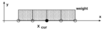
With Centered smoothing, the current Y-value has the highest weight, and the weight decreases linearly as the distance to the current X-value increases.
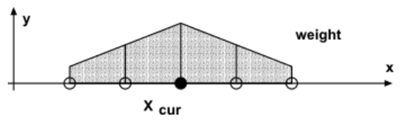
With Upwind smoothing, first consider the Y-value of the farthest neighboor. The side with the highest Y-value is weighted more (to the left or the right side of the current X-value).
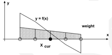
With Downwind smoothing, first consider the Y-value of the farthest neighboor. The side with the lowest Y-value is weighted more (to the left or the right side of the current X-value).
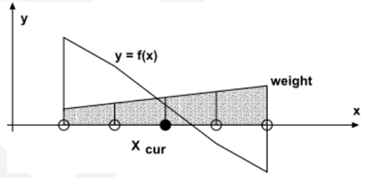
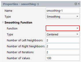
In the figure below, we see the effect of the smoothing on the density of probability of the ln(stretching), in a given slice: in blue the original curve, in red the smoothed curve.
Arithmetic on Sum Functions
With this method, it is possible to combine two sum functions with an arithmetic operator (addition, multiplication, division and subtraction). Select the two sum functions, the operator.
The calculation is performed as follows: for a given slice index i (that assumes that the two sum functions have been evaluated on the same slicing), we take the corresponding values of the two sum functions F1( i ) and F2 ( i ) and we create a new function Y: the value of the result function for slice index i will be :
Y(i) = F1( i ) <operator> F2( i )
This function is useful to evaluate the global efficiency of stretching (see annexe for further details).
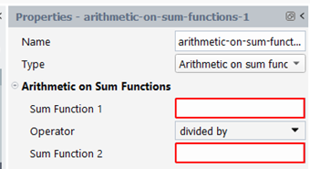
Distance Distribution
To calculate the evolution of the distribution function of distances between material points, you have to specify the slicing to be used, to select the coordinates quantity, to enter the number of values to represent the curves and to provide the maximum possible distance between pairs of points. Eventually, you have to choose between two modes of evaluation:
the first determines the distance distribution between all pairs of points. The maximum distance measured will be about the size of the flow domain, if the flow domain is closed.
the other determines the distance distribution only for pairs of points that are close neighboors (this is the default). The maximum distance measured, for a closed flow domain, will be

where V is the volume of the flow domain and n, the number of material points. The search of neighbouring points will be done only for distance between 0 and the value you specified. It is recommended that you choose a value greater than the maximum distance evaluated above.
For both modes: when evaluating the distance distribution for a given slice, we do not take into account pairs of points having a distance between them higher than this maximum.
If you manage to compare this distribution to another one, it is mandatory to use same settings for both functions. More particularly, if the domain is closed (as in a batch mixer), you have to compare a situation where all points are distributed randomly in the whole flow domain, with another one where the points are concentrated initially in a small box inside the flow domain. It is mandatory to have same number of material points for both cases, and same slicing. See paragraph 14 “Deviation function” for further details.
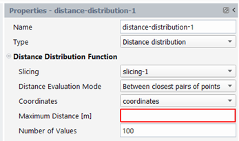
In the figure below, we plot the distance distribution functions for a few slices: you find the distance between pairs of points on the X axis and the distance distribution function on the Y axis
Distribution in Zones
To calculate the evolution of the distribution of material points initially concentrated in a box, specify two set of slices: the current slicing contains points coming from the real distribution (source=box), the optimal slicing contains points coming from an optimal distribution (source=flow domain). The coordinates quantity must be provided. Two ways exist to define the zones:
By boxes description: the user specifies the coordinates of the smallest box surrounding the flow domain and the number of times we divide that box in each axial direction (X, Y, Z). By default, the coordinates of the box corners are the one of the smallest box surrounding the full mesh. The number of zones in each direction is set to 2 by default.
By centers description: the user specifies the coordinates of the center of the zones in an ASCII file. The format of this file is as follows; on each line, there are the three coordinates (X,Y,Z) of one center. If the flow domain is 2D, the Z component is set to zero.
The panel appears like these for the 2 modes of Zones description:
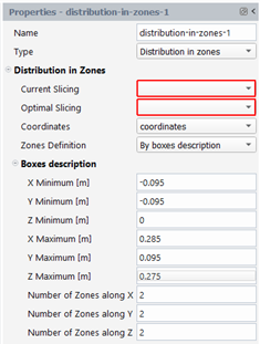
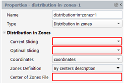
With this function, one obtains for each slice S:
the deviation of distribution for each zone Z:

(34–20)
where nbr(Z,S) and nbo(Z,S) are the number of points included in zone Z of the real and optimal distributions respectively, and nbtotr and nbtoto are the total number of points in the real and optimal distributions respectively.
If δ(Z,S) is zero, that means that the right number of points is included in zone Z.
If δ(Z,S) is negative, that means that the number of points included in that zone is smaller than the optimum: there is a local lack of points.
If δ(Z,S) is positive, that means that the number of points included in that zone is larger than the optimum: there is a local excess of points.
For visualization in charts, Fluent Materials Processing App generates curves named: <function-name>_zone<zone-id>.csv with <zone-id> ranged in interval [0, nbzones-1]. They contain the evolution along the slices of the deviation of distribution for the zone <zone-id>
the global index of distribution in zones:

A value of 1 means that the points are well concentrated in a small volume of the full fluid domain. While when we reach a value of 0, the points are well distributed in each zone of the flow domain.
For visualization in charts, Fluent Materials Processing App generates one curve named: <function-name>_global_index.csv that contains the evolution along the slices of the global index of distribution in zones.
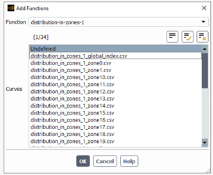
In the figure below, as an example, we plot the global index of distribution in zones along the slices and the deviation of distribution for a few zones.
Remark: as we compare two distributions of points, it is mandatory to have same number of material points for both sources, and same slicing. Moreover, the zones should not be too small (and their number huge), otherwise the computation time may increase excessively.
Points Concentration Deviation Function
This function allows you to calculate the deviation of points concentration in a slice compared to a perfect points concentration. This deviation is evaluated for each slice of the selected slicing. You must specify a slice and a coordinates quantity. Moreover, you must introduce the points concentration for a perfect distribution in each slice. This perfect distribution may be evaluated as follows:
For a 3D open flow domain, the slicing is done on space, in the direction of the flow; therefore, each slice will be a surface. It is assumed that each slice has the same perfect points concentration, which is equal to the number of points in a slice divided by the area of the part of the slice that cuts the flow domain.
For a 3D closed flow domain, one performs a slicing in time; therefore, each slice will be a volume. It is assumed that each slice has the same perfect points concentration, which is equal to the number of points tracked divided by the volume of the flow domain.
For a 2D open flow domain, the slicing is done on space, in the direction of the flow; therefore, each slice will be a line. It is assumed that each slice has the same perfect points concentration, which is equal to the number of points in a slice divided by the length of the part of the slice that cuts the flow domain.
For a 2D closed flow domain, one performs a slicing in time; therefore, each slice will be a surface. It is assumed that each slice has the same perfect points concentration, which is equal to the number of points tracked, divided by the area of the flow domain.
In order to evaluate the points concentration in each slice, one must specify the radius of the sample around each point; all points in the neighborhood of point x at a distance smaller than this radius will be taken to evaluate the local points concentration at position x. This radius must be chosen carefully; if it is too small, no points will be found and the local concentration will not be relevant; if it is too large, the concentration will be identical for all points in the slice and will not change from slice to slice. As a first estimation, we suggest to take as the radius a tenth of a typical distance in the slice (for example, the diameter of a rotor or of a screw).
One also has to specify the minimum number of points needed to evaluate the points concentration at a position x; the default is set to 3. If the number of neighboring points is smaller than this minimum, the sample radius is progressively increased (for that position only), until it has the correct number of neighbors.
Eventually, the dimensionality of the slices must be specified. If the slices are straight lines (dim=1), surfaces (dim=2) or volumes (dim=3). This is needed to evaluate the local points concentration
 : in a given slice S, for each point x, the number of neighbors Nx within a sample
radius R is determined. Depending on the dimensionality (dim) of the
slices, one can evaluate the local points concentration :
: in a given slice S, for each point x, the number of neighbors Nx within a sample
radius R is determined. Depending on the dimensionality (dim) of the
slices, one can evaluate the local points concentration :
The deviation of the points concentration in a slice S is evaluated as follows:

(34–21)
where N is the number of points in the slice
 corresponds to the location of point i in slice
 , and
, and  is the perfect points concentration.
Note that the points concentration is not evaluated in areas of the mixer that do not contain material points. If distributive mixing improves, the points concentration deviation should decrease. At perfect distribution, the same points concentration is found at any location in the slice and should be equal to the perfect points concentration, and the deviation
 should be null.
Note that if you enter a null perfect points concentration in 13,
 will be the average points concentration in slice S.
By this way, there is a mean of evaluating the perfect points
concentration if the methods given above are not suitable: to do so, in
a first “Points Concentration Deviation Function” object,
select a slicing object performed on an optimal distribution of points
and set the perfect points concentration to zero. After calculation, in
the corresponding chart, take the average value of
will be the average points concentration in slice S.
By this way, there is a mean of evaluating the perfect points
concentration if the methods given above are not suitable: to do so, in
a first “Points Concentration Deviation Function” object,
select a slicing object performed on an optimal distribution of points
and set the perfect points concentration to zero. After calculation, in
the corresponding chart, take the average value of  , noted here
  . Now, in a second “Points Concentration
Deviation Function” object, select a slicing object performed on
the real distribution of points and set the perfect points concentration
to
. Now, in a second “Points Concentration
Deviation Function” object, select a slicing object performed on
the real distribution of points and set the perfect points concentration
to  . The other properties of these two objects should be
the same.
. The other properties of these two objects should be
the same.The panel appears like this:
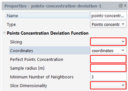
An example of the evolution of the deviation of the points concentration can be seen below (for the batch mixer GK7N):
Deviation Function
This function will allow you to calculate the gap existing between two density of probability functions. The first one has been obtained on a slicing performed on the real set of pathlines, while the second one has been obtained on a slicing performed on the optimal set of pathlines. There are three different methods to evaluate the deviation, δ, for a given slice <idx>:
Integral of differences:

Difference of the means:

Difference of the standard deviations:

Where

And

The panel appears like this:
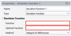
If you plan to measure how far is the current distance distribution (explained in paragraph 11 “Distance distribution”) to a perfect distance distribution, you need to define the following objects: 1. A “distance distribution” object (named “ddr”) defined on a slicing on the “real” set of pathlines (initially concentrated in a box, if domain is closed). 2. A “distance distribution” object (named “ddo”) defined on a slicing on the “optimal” set of pathlines (initially the whole flow domain, if domain is closed). 3. A “Deviation Function” defined on both “ddr” function and “ddo” optimal function. Use the default method “Integral of differences”. We call this function the “distribution index”. An example of the evolution of the distribution index can be seen below (for the batch mixer GK7N):
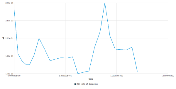
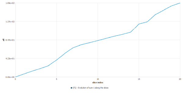
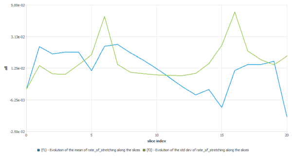
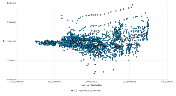
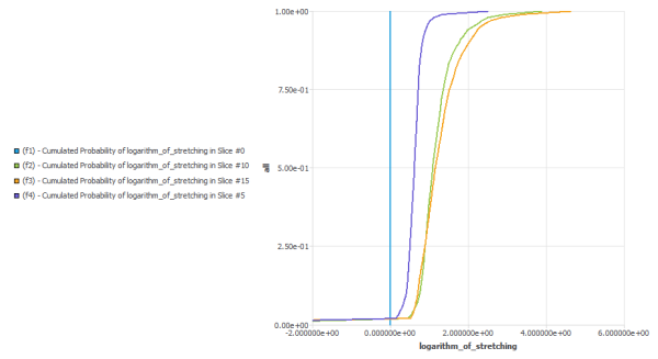
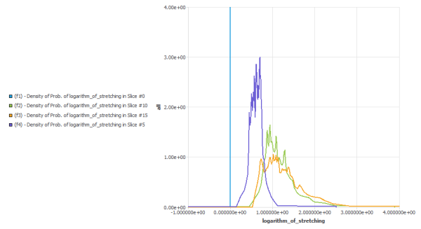
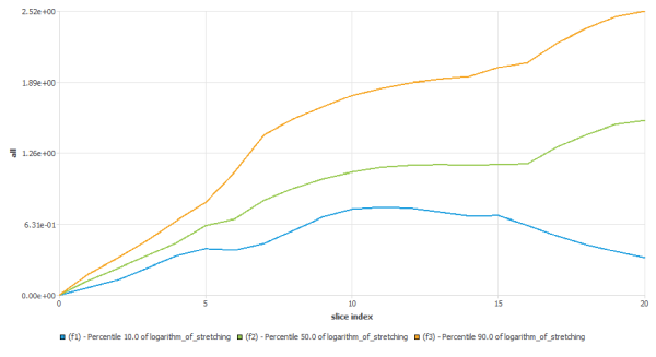
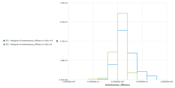
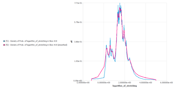
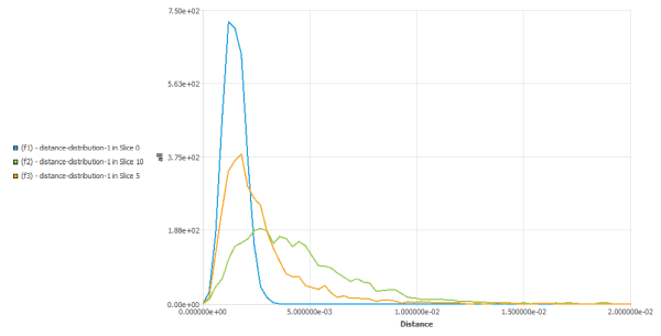
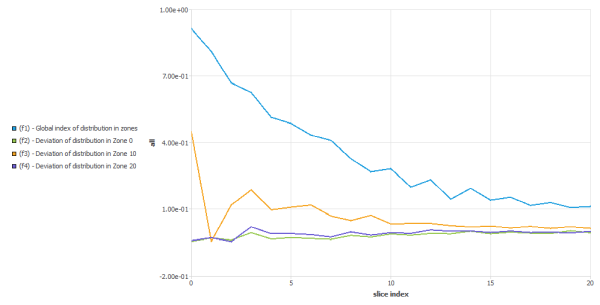
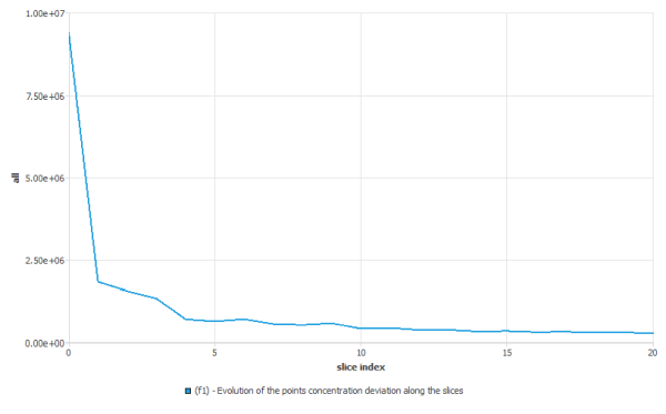
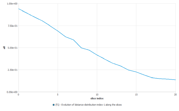
Once all statistical objects have been defined (pathlines sets, quantities, slicings, functions), one can compute effectively these objects. Click the Run Calculation item in the Outline view:
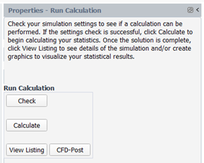
Or use the ribbon:
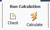
With the “Check” button, one will analyze the setup of the statistical task and provide error message(s) if something is ill posed or incomplete. If the check is successful, one can start the solver: click on Calculate. Polystat application will be run in the background and generate the requested files (outputs of pathlines sets, outputs of slicings, statistical curves). One can get a summary of this calculation by clicking on “View Listing” button: it will be printed in the Transcript page of the Graphics window. Let us mention that the naming of the objects may be different in Polystat and in Fluent Materials Processing App:
Pathlines set  Set of Trajectories
Quantity  Property
Slicing  Set of Slices
The statistical curves can be visualized in Fluent Materials Processing App, by creating Charts. Pathlines and Slicing can be visualized into CFD-Post (if their outputs were requested in the corresponding objects), by clicking CFD-Post icon in the ribbon (or the same button in the Run Calculation property panel):
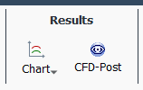
In each chart, the user has to specify which functions curves to add: to do so, one has to click on the “Add Function Curves” button, at the bottom of the property panel. Moreover, one can also add external curves to be plotted together with function curves: to do so, one has to click on the “Add External Curves” button, at the bottom of the same property panel. The “Function Curves” and “External Curves” properties are updated accordingly. It is possible to add a title to the chart and change the kind of axes (linear to log for both X and Y axes). Eventually, click on “Draw” button to visualize the chart (in the Plots page of the Graphics). It is also possible to save the current plot into a *.png file (“Save” button) and to modify the list of curves to draw (“Remove Curves” button)
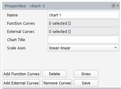
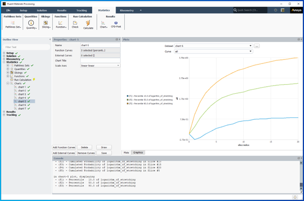
Weighting:
A weighting mode function of local flux is adequate for space slicing: by this way we "weight" more the material points that have higher normal velocity to the slice.
The general formula for the sum, the mean and the standard deviation of a quantity are:

where the index j indicates the j-th instant of slice i,
 is the value of quantity
  at instant j, and
 is the weight at instant j.
To calculate the probability function
 , the following set of pairs is sorted:
Finally the probability to find a value
 below
below  is:
is: 
where nbi is the number of instants in slice i.
The value of the weight is:
if no weighting:

if weighting everywhere:

where
 is the dot product of the velocity at
instant j by the normal of the slice i.
is the dot product of the velocity at
instant j by the normal of the slice i.Note: this should only be used if all the velocities in a slice have the same general direction (no backflow on a part of the slice).
if weighting when V.n is positive:

where
 is the dot product of the velocity at
instant j by the normal of the slice i.
is the dot product of the velocity at
instant j by the normal of the slice i.Note: we take into account and weight only the instants having their velocity in a slice in the same direction than the normal of the slice.
if weighting when V.n is negative:

where
 is the dot product of the velocity at
instant j by the normal of the slice i.
is the dot product of the velocity at
instant j by the normal of the slice i.Note: we take into account and weight only the instants having their velocity in a slice in the opposite direction to the normal of the slice.
Global efficiency of Stretching
Let's suppose the flow to be 2D, steady-state, in a closed domain: the mixing evolves thus with time. We will explain how we can calculate the time evolution of the global efficiency of stretching. This global efficiency of stretching can be defined as:

To calculate such a parameter, the following steps are necessary:
Along the pathlines are calculated the logarithm of stretching and the cumulated dissipation. Let us recall that the cumulated dissipation is defined as follows:

We perform a slicing on the time (N slices, every Δt seconds).
We calculate the sum function of the stretching on the time slicing:

We calculate the sum function of the cumulated dissipation <D> on the time slicing:

Finally, we divide the two sum functions to obtain the global efficiency of stretching:

Let us note that all functions based on stretching properties are theoretically dependent on the initial orientation M imposed at start of each material points. However, rapidly, as the mixing improves, the stretching properties are less and less affected by this initial condition.
[1] "Two-Dimensional Dynamic Study of the Distributive Mixing in an Internal Mixer". Intern. Polymer Proc.. 3–10. 1994.
[3] "Possibilities of Glass Tank Modeling for the Prediction of the Quality of Melting Processes". Ceram. Eng. Sci. Proc.. 139–160. 1993.