Once the report is generated, it appears in its own tab alongside the graphics window. Alternatively, you can use the View button in the Simulation Report task page for a selected report.
Note: Report settings for all generated reports will be saved with the case file. As long as
the FluentReportServer folder is not moved or deleted from the
working directory, you can read in a case file where you have previously generated a report
and immediately view the report using the View button
without needing to generate it again.
Use the hyperlinked table of contents to jump to different portions of the report.
- 45.4.1. Viewing System Information
- 45.4.2. Viewing Geometry and Mesh Information
- 45.4.3. Viewing Simulation Setup Information
- 45.4.4. Viewing Run Information
- 45.4.5. Viewing Solution Status
- 45.4.6. Viewing Named Expression Information
- 45.4.7. Viewing Report Definition Information
- 45.4.8. Viewing Plot Information
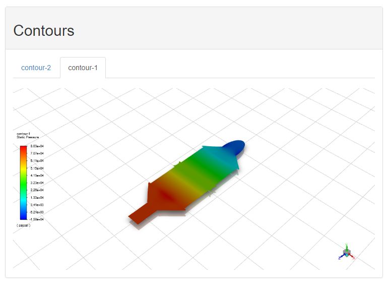
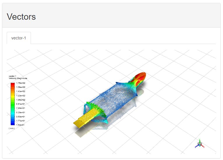
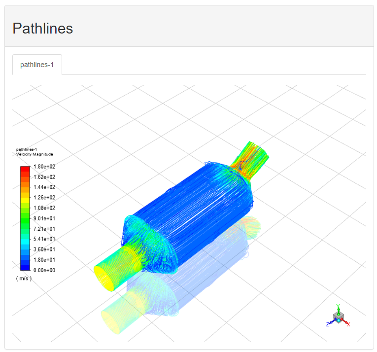
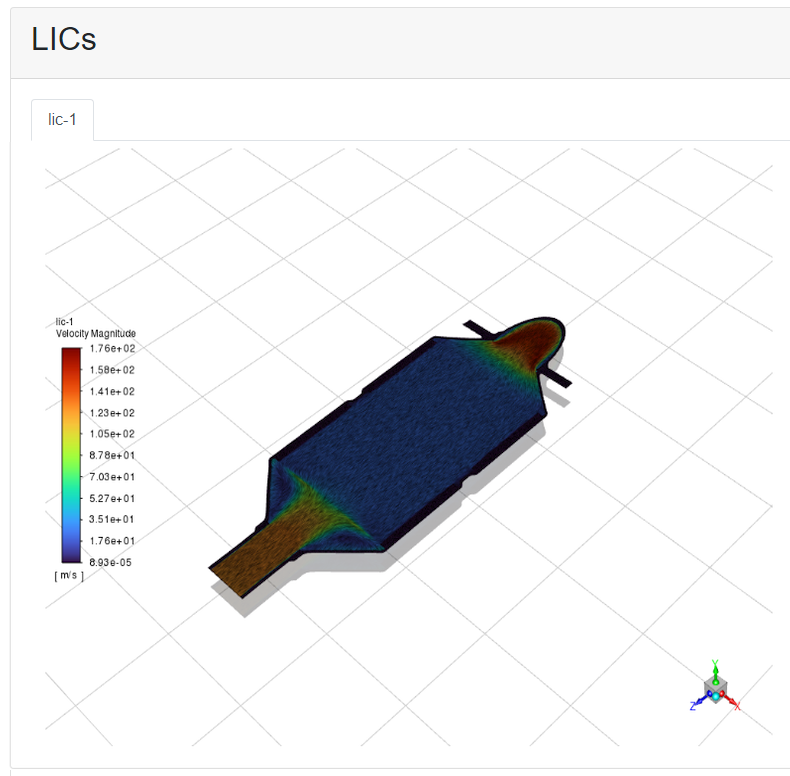
- 45.4.9. Viewing Contours, Vectors, Pathlines, LICs, XY Plots, Scenes, Histograms, and Animations
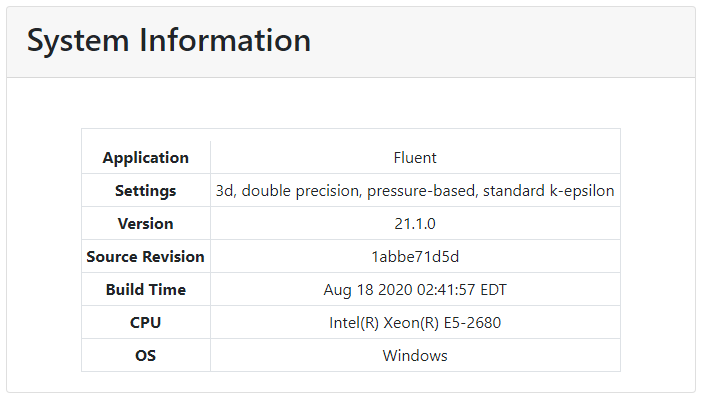
System Information information automatically includes details for the Application (the product name, such as Fluent), Settings (such as 3D, double-precision, etc.), Version (such as 20.2, etc.), Source Revision, Build Time, CPU, and OS.
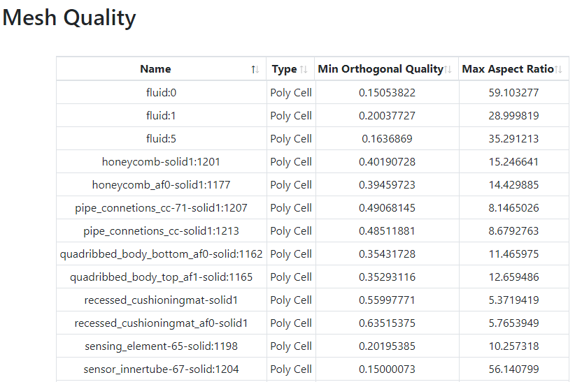
Geometry and Mesh information includes a default Mesh Quality table of the simulation's meshing statistics including: region names, their volume fill type, the minimum orthogonal quality, and the maximum aspect ratio.
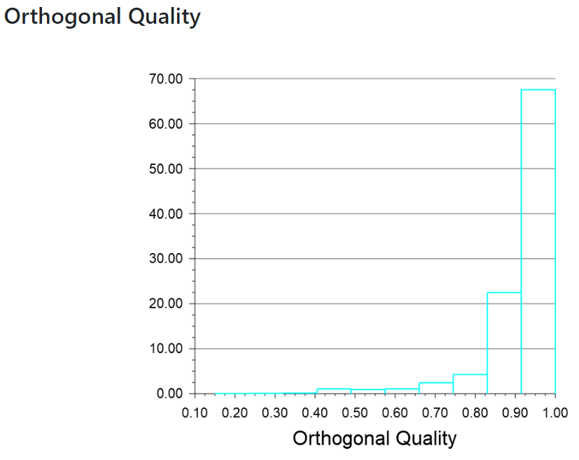
You are also presented with a default Orthogonal Quality chart.
Simulation Setup information includes the Solver Settings and Physics sections (which itself contains sections for Models, Material Properties, Cell Zone Conditions, and Boundary Conditions).
Note: Under Simulation Setup, the Show Only Modified Settings check box is enabled by default so that the report only displays settings that have been changed from the default values.
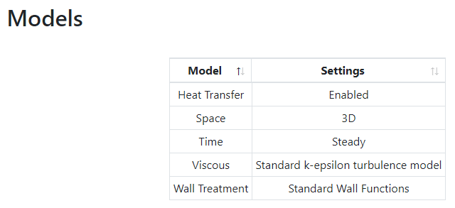
The Models section, under Physics, includes the numerical models that have been enabled in the simulation, such as the turbulence, heat transfer, etc.
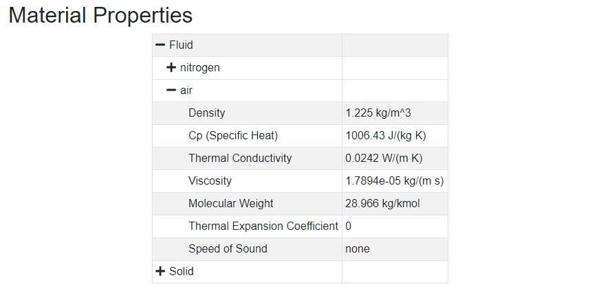
The Material Properties section, under Physics, includes the properties of the materials used in the simulation, such as the density, molecular weight, etc.
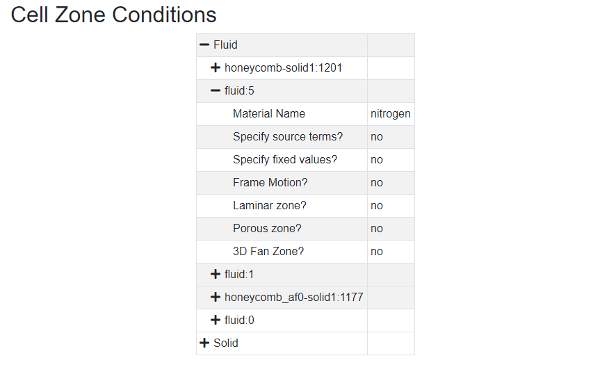
The Cell Zone Conditions section, under Physics, includes the specific setting for all cell zones (fluid and solid) used in the simulation, such as the material assignment, whether its a porous zone or not, whether there is motion or not, etc.
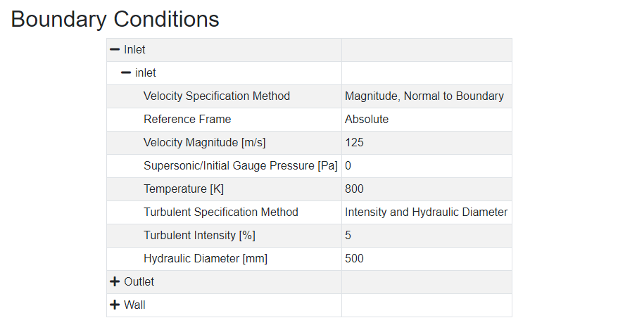
The Boundary Conditions section, under Physics, includes the specific setting for all boundaries (inlets, outlets, walls, etc.) used in the simulation, such as the velocity specification, temperature, etc.
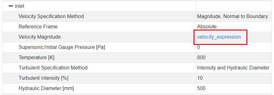
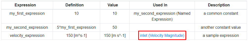
Note: If you use any named expressions as part of your boundary condition definitions, the named expressions are displayed in the Boundary Condition table as hyperlinks that take you to the Named Expressions section of the simulation report.
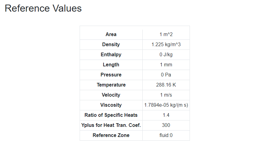
The Reference Values section, under Physics, includes the reference values for several key physics-related variables in your simulation, such as density, pressure, temperature, etc.
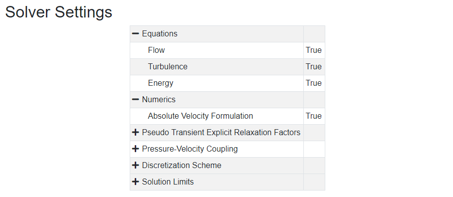
The Solver Settings section includes the numerical parameters of the simulation, such as the equations solved, discretization scheme, etc.
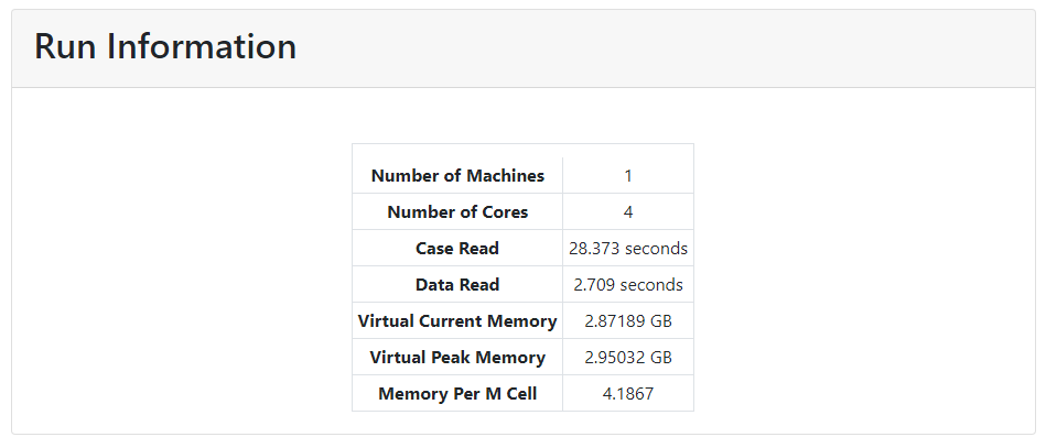
The Run Information section contains information such as the number of machines and cores used, memory usage, etc.
You also have the option of adding licensing information to your report by selecting the Include License Usage option.
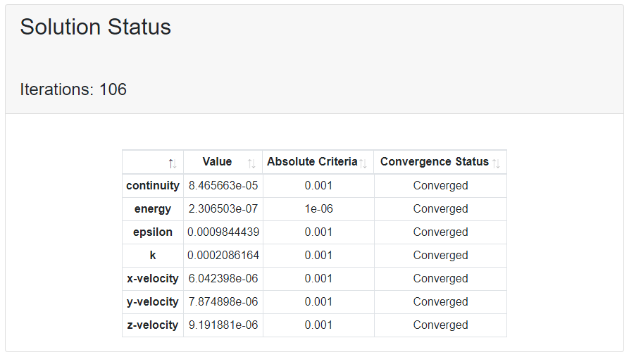
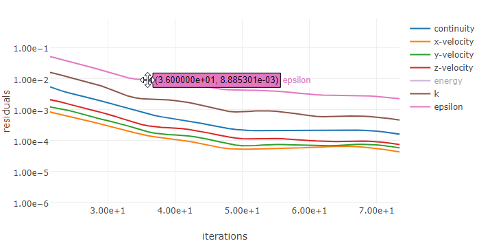
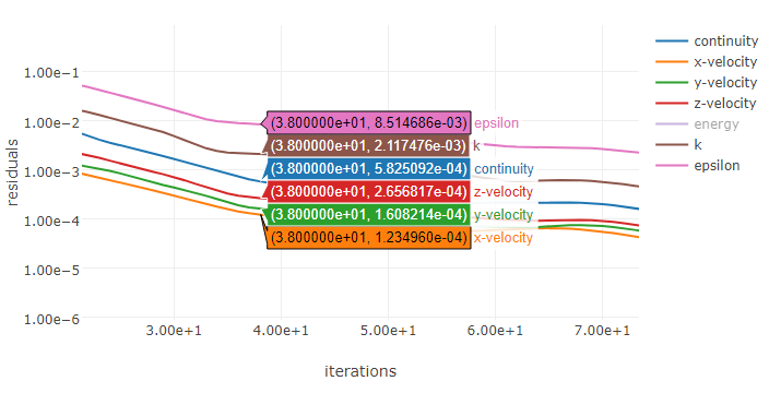
The Solution Status section contains information related to the simulation residuals and the convergence status.
The Named Expressions section includes a table of any named expressions from your simulation, along with their definitions, descriptions and where they are used
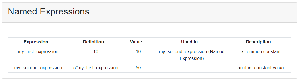
Note: Any named expressions that are utilized as boundary conditions are displayed in the Named Expressions table as hyperlinks that take you to the Boundary Conditions section of the simulation report.
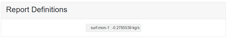
The Report Definitions section includes a table of any report definitions from your simulation.
The Plots section includes Residuals plots and Report Plots, if available in your simulation.
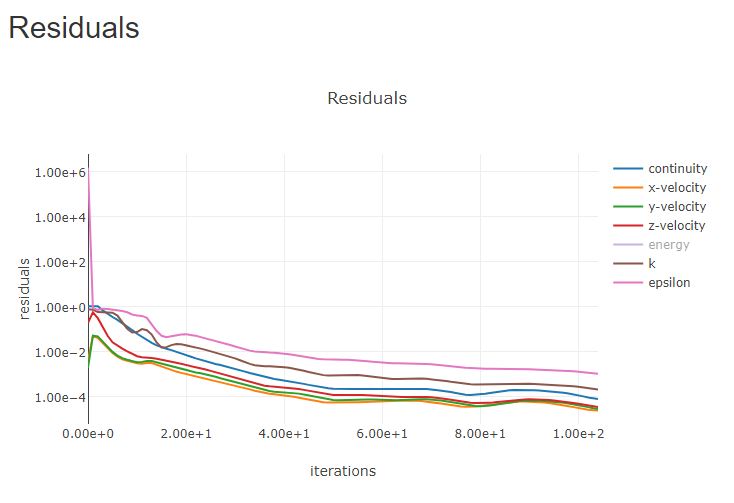
Note: You can adjust the visible range of the axes by clicking and dragging the mouse along the plot (vertically or horizontally).
Note: You can also zoom into the plot by clicking and dragging the mouse along the plot (diagonally).
There are several built-in features for viewing plot information, using the toolbar in the upper right-hand corner.
Download Plot as a PNG: allows you to save a copy of a plot as an image file. Specify the name and location of your file, or use the default name and location (the default location is your working folder).
Zoom: allows you to adjust the zoom level.
Pan: allows you to move vertically or horizontally across the plot.
Zoom in: allows you to zoom into the view.
Zoom out: allows you to zoom out of the view.
Autoscale: allows you to return to the view.
Reset axes: allows you to return to the original axis orientation.
Show closest data on hover: allows you to see specific data as you hover over the plot.
Compare data on hover: allows you to see and compare specific data as you hover over the plot.
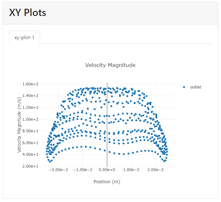
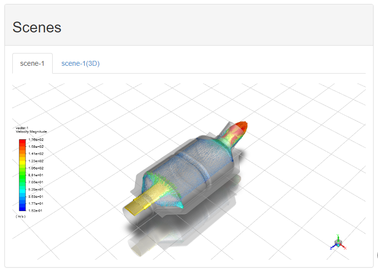
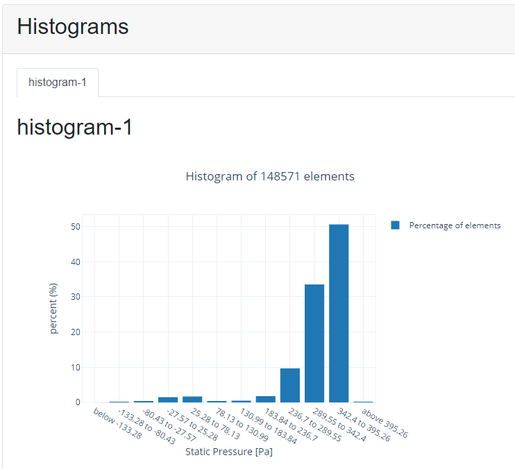
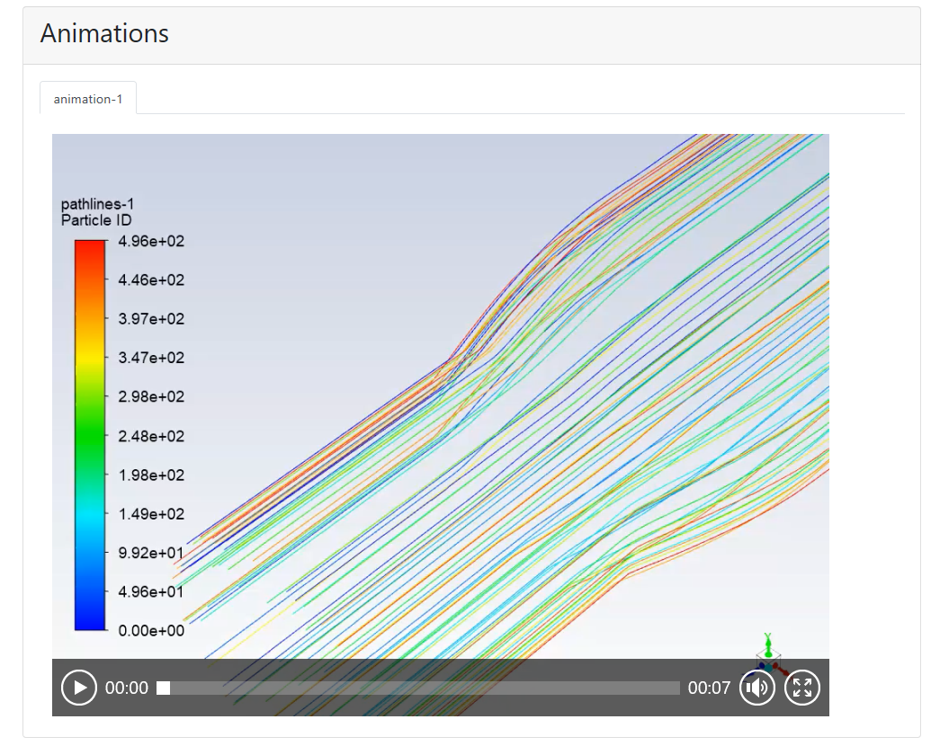
Graphical displays of Contours, Vectors, Pathlines, LICs, XY Plots, Scenes, Histograms, and Animations are able to be included in your report if they are available in your simulation.
Note: The layout of your results can also be arranged in a tabular format. See Changing the Layout of Your Results for details.
Note: AVZ animations are represented in your simulation report using static proxy images. You can play an embedded AVZ animation directly within your simulation report. Hovering over the static proxy image displays a 'play' button that you can then select to play the embedded animation.