


After you have completed your inputs and performed any coupled calculations, you can display the location of the fibers and source terms of the fibers, and you can write fiber data to files for further analysis of fiber variables.
The following data can be displayed using graphical and alphanumeric reporting facilities:
Graphical display of fiber locations
Exchange terms with surrounding fluid
Fiber solution variables.
For more information, see the following sections:
When you have defined fiber injections, as described in Defining Fibers, you can display the location of the fibers using Ansys Fluent’s Contour plot facility (Figure 34.14: Displaying Fiber Locations Using the Contours Dialog Box).
![]() Results → Graphics
→ Contours
Results → Graphics
→ Contours ![]() Edit...
Edit...
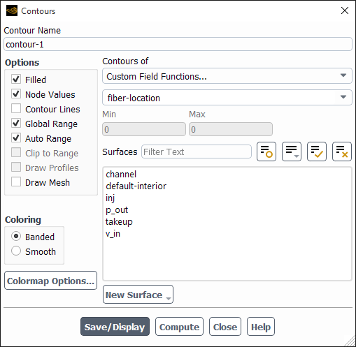
In the Contours of drop-down list, select Custom Field Functions..., then select fiber-location. The values in this field are between zero and the number of fiber cells in an Ansys Fluent grid cell.
You may generate iso-surfaces of constant values of fiber-location to display the fibers in 3D problems.
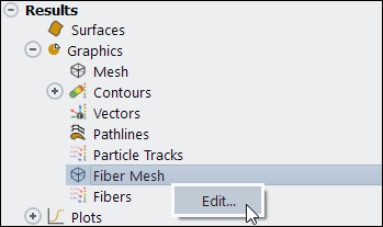
You can also display the locations of the fibers and their grid discretization using the Fiber Mesh Display dialog box, which can be accessed from the Results/Graphics/Fiber Mesh tree item.
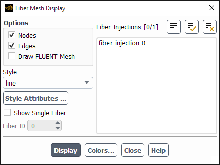
The following mesh discretization options are available:
Nodes: displays the end points of fiber volume cells
Edges: displays a line along the path of fibers in the domain
Draw Fluent mesh: Enables the display of the CFD mesh geometry with the mesh display settings specified in the Mesh Display dialog box. The Mesh Display dialog box will appear automatically when you enable the Draw Fluent mesh option.
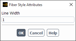
You can set the fiber Line Width in the Fiber Style Attribute dialog box accessed by clicking the Style Attributes... button.
For the injections selected in the Fiber Injections selection list, you can display either all injection fibers or single fibers with a specified Fiber ID (when the Show Single Fiber option is selected).
The continuous fiber model computes and stores the exchange of momentum, heat, mass, and radiation in each control volume in your Ansys Fluent model. You can display these variables graphically by drawing contours, profiles, and so on. They all are contained in the Custom Field Functions... category of the variable selection drop-down list that appears in postprocessing dialog boxes:
- fiber-mass-source
defined by Equation 22–22.
- fiber-x-momentum-source
is the x-component of the momentum exchange, defined by Equation 22–21.
- fiber-y-momentum-source
is the y-component of the momentum exchange, defined by Equation 22–21.
- fiber-z-momentum-source
is the z-component of the momentum exchange, defined by Equation 22–21.
- fiber-energy-source
defined by Equation 22–23.
- fiber-dom-absorption
defined by Equation 22–24.
- fiber-dom-emission
defined by Equation 22–25.
Note that these exchange terms are updated and displayed only when coupled computations are performed.
You can use Ansys Fluent’s Plot facilities to analyze fiber solution variables such as fiber velocity, temperature, diameter, and so on.
To investigate fiber variables you have to generate an xy-file for every variable using the following procedure from the text command interface (assuming that you have already defined a fiber injection):
Store an xy-file with the variable of interest.
continuous-fiber→print-xyEnter the fiber injection of interest when asked for
Fiber Injection name>Specify a variable for
x-column. This will be used as abscissa in the file plot.Specify another variable for
y-column, which will be used as ordinate in the file plot.Specify a file name when asked for
XY plot file name.Load the file with Ansys Fluent’s xy plot facilities, described in the Ansys Fluent manual.
The following variables can be entered as x-column and
y-column:
axial drag
conductivity
curvature
diameter
enthalpy
evaporated mass flux
heat transfer coefficient
lateral drag
length
mass flow
mass fraction
mass transfer coefficient
Nusselt number
Sherwood number
Reynolds number
specific heat
surface mass fraction
temperature
tensile force
user variable
velocity
velocity gradient
viscosity
If a fiber injection consists of several fibers, the data of all fibers in this fiber injection will be stored in the xy-file.
In addition to this, you can store a fiber history file for a fiber injection as described in Print Fiber Injections. This can be used to analyze a single fiber using Ansys Fluent xy-plot facilities or by external postprocessing programs.
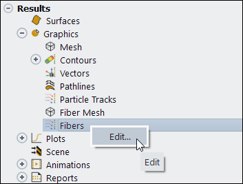
To visualize injection fibers, you can use the Fiber Display dialog box, which can be accessed from the Results/Graphics/Fibers tree item.
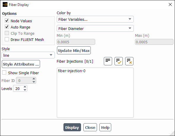
The Fiber Display dialog box offers the same display options as those in the Fiber Mesh Display dialog box (Figure 34.15: The Fiber Mesh Display Dialog Box). Similarly, for the injections selected in the Fiber Injections selection list, you can display either all injection fibers or single fibers with a specified Fiber ID (when the Show Single Fiber option is selected).
You can color the fibers by the fiber variables listed in XY Plots or by the following additional fiber variables:
Fiber ID
Fiber Density
Fiber Tension
You can control the smooth gradation of fiber colors by specifying the number of fiber Levels.
The Fiber Module can be used in serial as well as in parallel calculations. Simulations in parallel require no additional input. The fiber iterations are performed entirely on the host process, whereas the flow field is parallelized. As a result, the overall performance may be limited by the host process if the fiber calculations are more time-consuming than the parallel flow-field iterations. Therefore, when simulating a large number of fibers, it is recommended to spawn the host process on a suitable machine. Refer to Parallel Processing in the Fluent User's Guide for further information on how to set up parallel calculations.