For more information, see the following sections:
- 34.6.1. Overview
- 34.6.2. Fiber Injection Types
- 34.6.3. Working with Fiber Injections
- 34.6.4. Defining Fiber Injection Properties
- 34.6.5. Point Properties Specific to Single Fiber Injections
- 34.6.6. Point Properties Specific to Line Fiber Injections
- 34.6.7. Point Properties Specific to Matrix Fiber Injections
- 34.6.8. Define Fiber Grids
The primary inputs that you must provide for the continuous fiber model calculations in Ansys Fluent are the starting positions, mass flow rate, take up positions, and other parameters for each fiber. These provide the boundary conditions for all dependent variables to be solved in the continuous fiber model. The primary inputs are:
Start point (
 ,
,  ,
,  coordinates) of the fiber.
Number of fibers in group. Each defined fiber can represent a group of fibers that will be used only to compute the appropriate source terms of a group of fibers.
Diameter of the fiber nozzle,
 .
.Mass flow rate per nozzle to compute the velocity of the fiber fluid in the nozzle. The velocity is used as boundary condition for the fiber momentum equation.
Temperature of the fiber at the nozzle,
 .
.Solvent mass fraction of the fiber fluid in the nozzle. This value is used as boundary condition for the solvent continuity equation.
Take-up point (
 ,
,  ,
,  coordinates) of the fiber.
Velocity or force at take-up point to describe the second boundary condition needed for the fiber momentum equation (see Equation 22–4).
In addition to these parameters, you have to define parameters for the grid that is distributed between the start position and take-up point of the fibers. On this grid the dependent fiber variables are solved, by discretizing Equation 22–1, Equation 22–4, and Equation 22–11.
You can define any number of different sets of fibers provided that your computer has sufficient memory.
You will define boundary conditions and grids for a fiber by creating a fiber “injection” and assigning parameters to it. In the continuous fiber model the following types of injections are provided:
single
Use this option to define a single fiber.
line
Use this option when the fibers you want to define start from a line and the starting points are located at constant intervals on this line.
matrix (only in 3D)
Use this option when the fiber starting points are arranged in the shape of a rectangle.
file
Use an ASCII file for entering coordinates and material properties of individual fiber injections in a tabular format as shown below.
;  1st commentary line
;  2nd commentary line
;  m-th commentary line
x1   y1   z1   df1   m1   Tf1   Ys1
x2   y2   z2   df2   m2   Tf2   Ys2
... ...  ...  ...  ...  ...  ...
xn   yn   zn   dfn   mn   Tfn   Ysn
where each injection is described by the following data fields, all on one line, separated by spaces:
x, y, and z are the Cartesian coordinates of the injection point. The z coordinate must be included for both 3D and 2D solvers to maintain the sequence in which the data entries are interpreted, however, the z coordinate is not used in 2D.
df is the fiber diameter
m is the mass flow rate
Tf is the temperature Ys is the solvent liquid mass fraction (ignored for melt spinning) You can include an arbitrary number of comments anywhere in the file. Commentary lines must begin with a semicolon (
;).
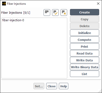
You will use the Fiber Injections dialog box (Figure 34.2: The Fiber Injections Dialog Box) to create, modify, copy, delete, initialize, compute, print, read, write, and list fiber injections. To access the Fiber Injections dialog box, first make sure you enable a fiber model, then go to
![]() Setup → Models →
Fiber-Injections
Setup → Models →
Fiber-Injections ![]() Edit...
Edit...
To create a fiber injection, click . A new fiber injection appears in the Fiber Injections list and the Set Fiber Injection Properties dialog box opens automatically to enable you to specify the fiber injection properties (as described in Point Properties Specific to Single Fiber Injections).
To modify an existing fiber injection, select its name in the Fiber Injections list and click . The Set Fiber Injection Properties dialog box opens, and you can modify the properties as needed.
To copy an existing fiber injection to a new fiber injection, select the existing injection in the Fiber Injections list and click . The Set Fiber Injection Properties dialog box will open with a new fiber injection that has the same properties as the fiber injection you have selected. This is useful if you want to set another injection with similar properties.
You can delete a fiber injection by selecting its name in the Fiber Injections list and clicking .
To initialize all solution variables of the fibers defined in a fiber injection, select its name in the Fiber Injections list and click . The solution variables will be set to the boundary condition values at the starting points of the fibers.
You can select several fiber injections when you want to initialize several fiber injections at one time.
Important: If you do not select a fiber injection and click , all fiber injections will be initialized.
To solve the fiber equations of a fiber injection for a number of iterations, select its name in the Fiber Injections list and click . The solution variables of the fibers defined in this fiber injection will be updated for the number of iterations specified in Figure 34.13: Fiber Solution Controls Dialog Box.
You can select several fiber injections when you want to compute several fiber injections at one time.
Important: If you do not select a fiber injection and click , all fiber injections will be computed.
To print the fiber solution variables of a fiber injection into a file, select its name in the Fiber Injections list and click . A file name is generated automatically based on the name of the fiber injection and the number of the fiber. The solution variables of each fiber is stored in a separate file. You may use this file for an external postprocessing or analysis of fiber data.
You can select several fiber injections when you want to print several fiber injections at one time.
Important: If you do not select a fiber injection and click , all fiber injections will be printed.
To read the data (properties and solution variables) of a fiber injection previously stored in a file, click . A file selection dialog box is opened where you can select the name of the file in a list or you can enter the file name directly. The names of all fiber injections included in the file are compared with the fiber injections already defined in the model. If the fiber injection exists already in your model, you are asked to overwrite it.
While the settings of the continuous fiber model for numerics and models are stored in the Ansys Fluent case file, the data of the fibers and defined injections have to be stored in a separate file. To write the data of a fiber injection to a file, click . A file selection dialog box is opened where you can select the name of an existing file to overwrite it or you can enter the name of a new file.
You can select several fiber injections when you want to store several fiber injections in one file.
Important: If you do not select a fiber injection and click , all fiber injections will be stored in the specified file.
To write the data of a fiber injection in binary format to a file, click . A file selector dialog box is opened where you can select the name of an existing file to overwrite it or you can enter the name of a new file.
You can select several fiber injections when you want to store several fiber injections in binary format in one file.
Important: If you do not select a fiber injection and click , all fiber injections will be stored in binary format in the specified file.
To list starting positions and boundary conditions of the fibers defined in a fiber injection, click . Ansys Fluent displays a list in the console window. For each fiber you have defined, the list contains the following (in SI units):
File number in the injection in the column headed
(NO). ,
,  , and
, and  position of the starting point in the columns headed
(X),(Y), and(Z).Fiber velocity in the column headed
(U).Temperature in the column headed
(T).Solvent mass fraction in the column headed
(SOLVENT).Diameter in the column headed
(DIAM).Mass flow rate in the column headed
(MFLOW).The number of fibers represented by this fiber group in the column headed
(FIBERS).The number of fiber grid cells defined for this fiber in the column headed
(CELLS).A notification whether the starting point of the fiber is located inside or outside the domain in the column headed
(IN DOMAIN?).
The boundary conditions at the take up point are also listed. This list consists of the following (in SI units):
 ,
,  , and
, and  position of the take-up point in the columns headed
(X),(Y), and(Z).Boundary condition type and its specified value (
VELOCITYfor given take-up velocity,FORCEfor given force in the fiber) in the column headed(BOUNDARY CONDITION).
You can select several fiber injections when you want to list several fiber injections.
Important: If you do not select a fiber injection and click , all fiber injections will be listed.
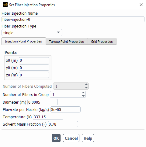
Once you have created an injection (using the Fiber Injections dialog box, as described in Creating Fiber Injections), you will use the Set Fiber Injection Properties dialog box (Figure 34.3: The Set Fiber Injection Properties Dialog Box) to define the fiber injection properties. (Remember that this dialog box opens when you create a new fiber injection, or when you select an existing fiber injection and click in the Fiber Injections dialog box.)
The procedure for defining a fiber injection is as follows:
If you want to change the name of the fiber injection from its default name, enter a new one in the Fiber Injection Name field. This is recommended if you are defining a large number of injections so you can easily distinguish them.
Choose the type of fiber injection in the Fiber Injection Type drop-down list. The three choices (single, line, and matrix) are described in Fiber Injection Types.
Click the Injection Point Properties tab (the default), and specify the point coordinates according to the fiber injection type, as described in Point Properties Specific to Single Fiber Injections–Point Properties Specific to Matrix Fiber Injections.
If each of the defined fibers is referring to a group of fibers, enter the number of fibers in Number of Fibers in Group. If your nozzle plate has 400 holes and you can simulate them as a line fiber injection with 5 groups, you have to enter a value of 80. This means that only 5 fibers are solved numerically, but each of these fibers stands for 80 fibers to be used to compute the source terms for the surrounding fluid. This enables you to reduce computing efforts while achieving a proper coupling with the surrounding fluid.
Important: Note that the Number of Fibers in Group is applied to all fibers, defined in your injection. If the number of fiber groups in your line or matrix injection is not the same for all fibers in this injection, you should split this injection into several fiber injections.
Specify the diameter of the nozzle in the Diameter field.
Enter the mass flow rate for a single nozzle in the Flow rate per Nozzle field. This will be used to compute the starting velocity of the fiber fluid.
Important: Note that the value specified refers to one single nozzle and not to the mass flow rate of all fibers defined in this fiber injection.
Specify the temperature of the fiber fluid leaving the nozzle in the Temperature field.
If you are modeling dry spun fibers you also have to enter the solvent’s mass fraction at the nozzle in the Solvent Mass Fraction field.
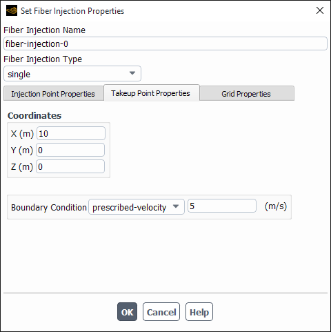
Click the Takeup Point Properties tab and enter the coordinates of the take-up point (see Figure 34.4: The Set Fiber Injection Properties Dialog Box With Take-Up Point Properties).
Important: Note that all fibers defined in the fiber injection are collected at the same point. If the fibers of your line or matrix injection vary in this property, you have to define them using several fiber injections.
Select the appropriate boundary condition from the Boundary Condition drop-down list and specify the value for this boundary condition. Choose prescribed-velocity if you know the drawing velocity (also called take-up velocity). Choose tensile-force with a value of zero if you want to simulate free falling fibers at the take-up point.
Click the Grid Properties tab and enter all data needed to generate the fiber grid as described in Define Fiber Grids.
For a single fiber injection, you have to specify the coordinates of the starting point
of the fiber. Click the Injection Point Properties tab and set the
 ,
,  , and
, and  coordinates in the x0, y0, and
z0 fields of the Points box.
(z0 will appear only for 3D problems.)
coordinates in the x0, y0, and
z0 fields of the Points box.
(z0 will appear only for 3D problems.)
In a line fiber injection the starting points of the fibers are arranged on a line at a
constant distance (see Figure 34.5: Line Injections). You have to specify
the coordinates of the starting point and the end point of this line. Click the
Injection Point Properties tab in the Set Fiber Injection
Properties dialog box (Figure 34.3: The Set Fiber Injection Properties Dialog Box). In the
Points region, set the  ,
,  , and
, and  coordinates in the x0, y0, and
z0 fields for the starting point of the line and the
coordinates in the x0, y0, and
z0 fields for the starting point of the line and the  ,
,  , and
, and  coordinates in the x1, y1, and
z1 fields for the end point of the line. (z0 and
z1 will appear only for 3D problems.)
coordinates in the x1, y1, and
z1 fields for the end point of the line. (z0 and
z1 will appear only for 3D problems.)
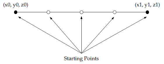
In addition to the coordinates, you have to set the number of fibers defined in the line injection by entering the appropriate value in the Point Density Edge1 field. See Figure 34.5: Line Injections for an example of a line fiber injection with a Point Density Edge1 of 5.
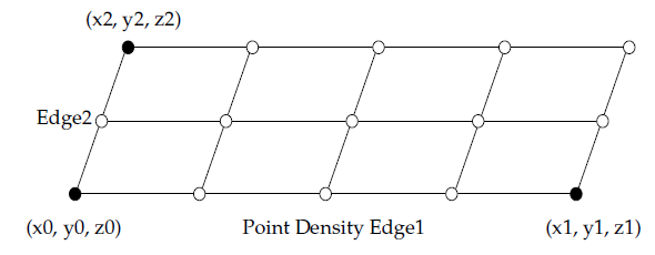
In a matrix fiber injection the starting points of the fibers are arranged in several rows having the shape of a rectangle or a parallelogram. Each row has the same distance to the previous and is divided into equal sections (see Figure 34.6: Matrix Injections).
You have to specify the coordinates of the starting point and the end of point of the
first row and the coordinates where the last row should start. Click the Injection
Point Properties tab in the Set Fiber Injection Properties
dialog box (Figure 34.3: The Set Fiber Injection Properties Dialog Box). In the
Points region, set the  ,
,  , and
, and  coordinates in the x0, y0, and
z0 fields for the starting point and the
coordinates in the x0, y0, and
z0 fields for the starting point and the  ,
,  , and
, and  coordinates in the x1, y1, and
z1 fields for the end point of the first row of fibers. The
coordinates in the x1, y1, and
z1 fields for the end point of the first row of fibers. The
 ,
,  , and
, and  coordinates of the starting point of the last row have to be entered in
the x2, y2, and z2
fields.
coordinates of the starting point of the last row have to be entered in
the x2, y2, and z2
fields.
At each row, the number of fibers specified in the Point Density Edge1 field are injected. The number of rows to be injected is specified in Edge2.
You can double check the number of fibers computed in this fiber injection if you inspect the Numbers of Fibers Computed field.
Important: Note that this fiber injection type is only available for 3D problems.
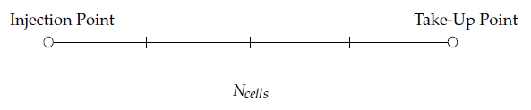
Each fiber consists of a straight line between the injection point and the take-up point. It is divided into a number of finite volume cells. Every fiber defined in a fiber injection has its own grid, which you can specify if you click the Grid Properties tab in the Set Fiber Injection Properties dialog box.
To define an equidistant grid for the fibers select equidistant from the Grid Type drop-down list. Specify the Number of Cells into which every fiber of the fiber injection will be divided.
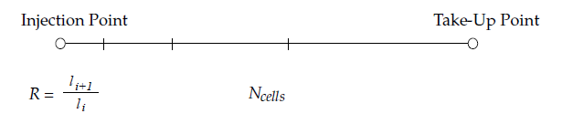
A one-sided grid is graded near the injection point of the fiber. To define a
one-sided grid for the fibers select one-sided from the
Grid Type drop-down list. Specify the Number of
Cells into which every fiber of the fiber injection will be divided. In
addition, you have to specify the ratio,  , between each subsequent fiber cell in the Grid Growth Factor
at Injection Point field. Values larger than 1 refine the grid, while values
smaller than 1 coarsen the grid.
, between each subsequent fiber cell in the Grid Growth Factor
at Injection Point field. Values larger than 1 refine the grid, while values
smaller than 1 coarsen the grid.
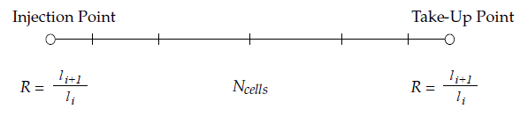
A two-sided grid is graded near the injection point as well as at the take-up point of
the fiber. To define a two-sided grid for the fibers, select
two-sided from the Grid Type drop-down list.
Specify the Number of Cells into which every fiber of the fiber
injection will be divided. You also have to specify the ratio,  , between each subsequent fiber cell at the injection point in the
Grid Growth Factor at Injection Point field and the ratio,
, between each subsequent fiber cell at the injection point in the
Grid Growth Factor at Injection Point field and the ratio,
 , near the take-up point in the Grid Growth Factor at Takeup
Point field. Values larger than 1 refine the grid, while values smaller than
1 will coarsen it.
, near the take-up point in the Grid Growth Factor at Takeup
Point field. Values larger than 1 refine the grid, while values smaller than
1 will coarsen it.
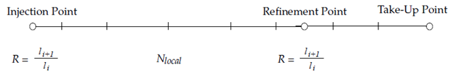
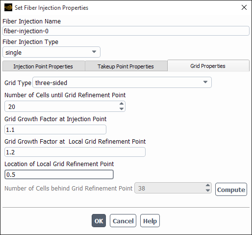
A three-sided grid consists of three sides where the fiber grid can be graded. The first side is near the injection point. The other two sides are around a refinement point within the fiber grid. Both sides at the refinement point are graded at the same ratio between the fiber grid cell lengths. To define a three-sided grid for the fibers, select three-sided from the Grid Type drop-down list (see Figure 34.11: Defining a Three-Sided Fiber Grid Using the Set Fiber Injection Properties Dialog Box). Specify the Number of Cells until Grid Refinement Point, the Grid Growth Factor at Injection Point, and the Grid Growth Factor at Local Grid Refinement Point. You also have to specify the location of the grid refinement point in the Location of Local Grid Refinement Point field in a dimensionless way. The value you have to enter is relative to the fiber length and may be between 0 and 1. Values larger than 1 refine the grid, while values smaller than 1 coarsen the grid.
Click the Compute button to estimate the Number of Cells behind Grid Refinement Point.