Geometry-based adaption works on the principle of geometry reconstruction. In this approach, the cell count of the mesh is increased by creating the new nodes in the domain in between the existing nodes of the mesh. The newly created nodes are projected in such a way that the resulting mesh is finer and has a shape that is closer to the original geometry.
The following sections explain how nodes are projected and the parameters that control the node propagation.
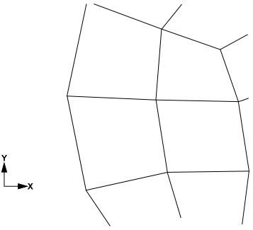
Consider a coarse mesh created for a circular geometry. A section of the mesh close to the circular edge is shown in Figure 24.5: Mesh Before Adaption. The edge is not smooth and has sharp corners, such that its shape does not closely resemble that of the original geometry. Using boundary adaption along with the geometry reconstruction option will result in a mesh with smoother edges, as shown in Figure 24.6: Projection of Nodes.
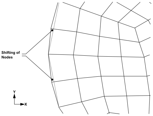
In Figure 24.6: Projection of Nodes, the dotted lines represent the original edge of the mesh. The boundary adaption process creates new nodes in between the original nodes. These nodes are projected towards the edge of the geometry, and as a result the resulting mesh has smooth edges and its shape is closer to the original geometry.
Important: Only the nodes created in the adaption process (newly created nodes) are projected; the original nodes retain their positions.
When using the PUMA adaption method (which is the default for 3D), you can control the node projection / displacement using the following:
auxiliary geometry definitions, which can be defined using a shape primitive, a user-defined function, a surface mesh, or a smooth background model reconstructed from the current node coordinates of one or more specified boundary zones (as described in Managing Auxiliary Geometry Definitions in the Fluent User's Guide)
an exponent that controls the degree to which the boundary displacement is also applied to the prismatic boundary layers adjacent to the surface (as described in Refining and Coarsening in the Fluent User's Guide)
For the hanging node adaption method, the following parameters control node projection and are specified in the Geometry Based Adaption Dialog Box.
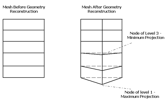
Levels of Projection Propagation: This parameter allows you to specify the number of node layers across which node propagation should take place for geometry reconstruction. A value of
1means only the nodes at the boundary will be projected, a value of2means the nodes at the boundary and the nodes in the next layer will be projected, and so on.Note: The nodes in the first level are projected by a maximum magnitude and the node in the last level are projected by a minimum magnitude. The magnitude of projection decreases gradually from the first level to the last level.
For example, a value of
3for Levels of Projection Propagation means, the level 1 node is projected by maximum magnitude and level 3 node is projected by minimum magnitude. Figure 24.7: Levels Projection Propagation and Magnitude illustrates the level of propagation and magnitude of projection of newly created nodes.Direction of Projection: This parameter allows you to specify the direction, X, Y, or Z (for 3D), for node projection. If you do not specify any direction, the node projection takes place at the nearest point of the newly created node.
Background Mesh: This option allows you to use a fine surface mesh as a background mesh, which is then used to reconstruct the geometry. When you read the surface mesh, the node projection will take place based on the node positions of the background mesh.
This option is useful when the mesh you want to adapt is very coarse and geometry is highly curved. In such cases, node projection, only by specifying the parameters may not result in a good quality mesh. However, you can also modify the propagation criteria by specifying the parameters.
Important: You can read only one surface mesh at a time. The various zones of the surface mesh will be listed in the Background Mesh drop-down list.
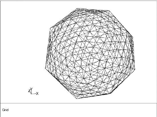
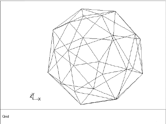
Consider a mesh created for a spherical geometry. The initial mesh is very coarse, resulting in sharp corners (as in Figure 24.8: Coarse Mesh of a Sphere). It does not represent the spherical geometry accurately. You can recover the original spherical geometry from this coarse mesh by using geometry-based adaption.
If you adapt boundaries of the domain without enabling the Reconstruct Geometry option, the resulting mesh (see Figure 24.9: Adapted Mesh Without Geometry Reconstruction) has a sufficient number of cells, but the boundary of the domain still contains sharp corners.
Boundary adaption only creates new nodes in between the existing nodes to increase the cell count of the mesh. Since it does not project the nodes, the shape of the mesh remains as it is.
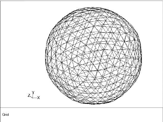
If you adapt the boundary with the Reconstruct Geometry option enabled, the resulting mesh (Figure 24.10: Mesh after Geometry-Based Adaption) has more cells and less sharp corners at the boundary. In addition, the newly created nodes are projected in a direction such that its shape is closer to the original geometry (that is, a sphere with smooth boundary).