Chapter 25: Modeling Solidification

This tutorial is divided into the following sections:

25.1. Introduction

This tutorial illustrates how to set up and solve a problem involving solidification and will demonstrate how to do the following:

Define a solidification problem.
Define pull velocities for simulation of continuous casting.
Define a surface tension gradient for Marangoni convection.
Solve a solidification problem.

25.2. Prerequisites

This tutorial is written with the assumption that you have completed the introductory tutorials found in this manual and that you are familiar with the Ansys Fluent outline view and ribbon structure. Some steps in the setup and solution procedure will not be shown explicitly.

25.3. Problem Description

This tutorial demonstrates the setup and solution procedure for a fluid flow and heat transfer problem involving solidification, namely the Czochralski growth process. The geometry considered is a 2D axisymmetric bowl (shown in Figure 25.1: Solidification in Czochralski Model), containing liquid metal. The bottom and sides of the bowl are heated above the liquidus temperature, as is the free surface of the liquid. The liquid is solidified by heat loss from the crystal and the solid is pulled out of the domain at a rate of 0.001 and a temperature of 500 . There is a steady injection of liquid at the bottom of the bowl with a velocity of and a temperature of 1300 . Material properties are listed in Figure 25.1: Solidification in Czochralski Model.

Starting with an existing 2D mesh, the details regarding the setup and solution procedure for the solidification problem are presented. The steady conduction solution for this problem is computed as an initial condition. Then, the fluid flow is enabled to investigate the effect of natural and Marangoni convection in a transient fashion.

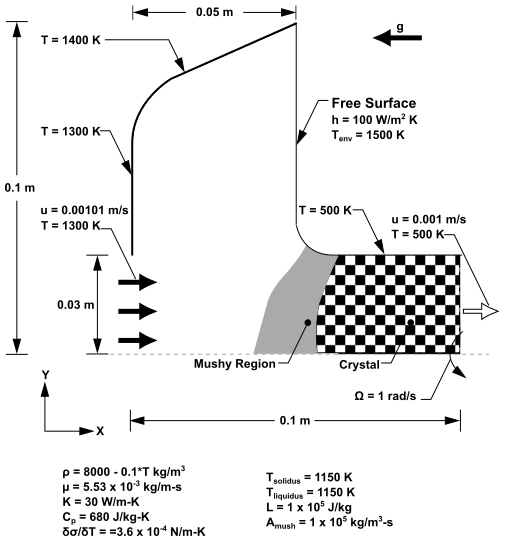
Figure 25.1: Solidification in Czochralski Model

In the above figure, is the mushy zone constant.

25.4. Setup and Solution

The following sections describe the setup and solution steps for this tutorial:

25.4.1. Preparation

To prepare for running this tutorial:

Download the solidification.zip file here .
Unzip solidification.zip to your working directory.
The mesh file solid.msh can be found in the folder.
Use the Fluent Launcher to start Ansys Fluent.
Select Solution in the top-left selection list to start Fluent in Solution Mode.
Select 2D under Dimension.
Disable Double Precision under Options.
Set Solver Processes to 1 under Parallel (Local Machine).

25.4.2. Reading and Checking the Mesh

Read the mesh file solid.msh.
File → Read → Mesh...
As the mesh is read by Ansys Fluent, messages will appear in the console reporting the progress of the reading.
A warning about the use of axis boundary conditions is displayed in the console. You are asked to consider making changes to the zone type or change the problem definition to axisymmetric. You will change the problem to axisymmetric swirl later in this tutorial.
Check the mesh.
Domain → Mesh → Check → Perform Mesh Check
Ansys Fluent will perform various checks on the mesh and will report the progress in the console. Make sure that the minimum volume is a positive number.
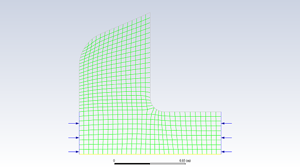
Examine the mesh (Figure 25.2: Mesh Display).
Figure 25.2: Mesh Display

25.4.3. Specifying Solver and Analysis Type

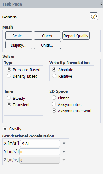
Select Axisymmetric Swirl from the 2D Space list and include the effects of gravity on the model.
Setup → General → Gravity
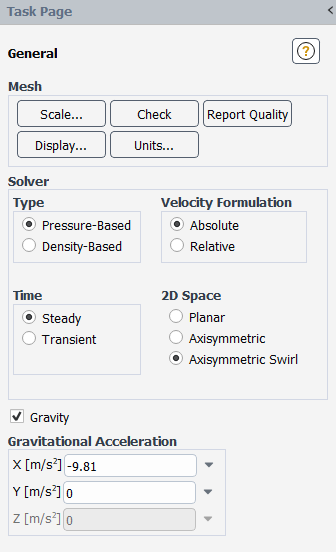
The geometry comprises an axisymmetric bowl. Furthermore, swirling flows are considered in this problem, so the selection of Axisymmetric Swirl best defines this geometry.
Also, note that the rotation axis is the X axis. Hence, the X direction is the axial direction and the Y direction is the radial direction. When modeling axisymmetric swirl, the swirl direction is the tangential direction.
1. Enable Gravity.
2. Enter -9.81 for X in the Gravitational Acceleration group box.

25.4.4. Specifying the Models

Enable the laminar viscous model.
Setup → Models → Viscous Edit...
1. Select Laminar in the Model group box.
Define the solidification model.
Setup → Models → Solidification & Melting Edit...
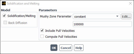
1. Enable the Solidification/Melting option in the Solidification and Melting dialog box.
  The Solidification and Melting dialog box will expand to show the related parameters.
2. Retain the default value of 100000 for the Mushy Zone Constant.
  This default value is acceptable for most cases.
3. Enable the Include Pull Velocities option.
  By including the pull velocities, you will account for the movement of the solidified material as it is continuously withdrawn from the domain in the continuous casting process.
  When you enable this option, the Solidification and Melting dialog box will expand to show the Compute Pull Velocities option. If you were to enable this additional option, Ansys Fluent would compute the pull velocities during the calculation. This approach is computationally expensive and is recommended only if the pull velocities are strongly dependent on the location of the liquid-solid interface. In this tutorial, you will patch values for the pull velocities instead of having Ansys Fluent compute them.
  For more information about computing the pull velocities, see the Fluent User's Guide.
4. Click OK to close the Solidification and Melting dialog box.
  An Information dialog box opens, telling you that available material properties have changed for the solidification model. You will set the material properties later, so you can click OK in the dialog box to acknowledge this information.
Note: Ansys Fluent will automatically enable the energy calculation when you enable the solidification model, so you need not visit the Energy dialog box.

25.4.5. Defining Materials

In this step, you will create a new material and specify its properties, including the melting heat, solidus temperature, and liquidus temperature.

Define a new material.
Setup → Materials → Fluid → air Edit...
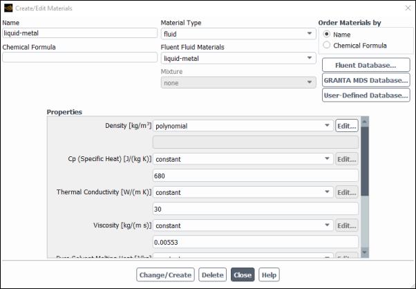
1. Enter liquid-metal for Name.
2. Select polynomial from the Density drop-down list in the Properties group box.
3. Configure the following settings In the Polynomial Profile dialog box:
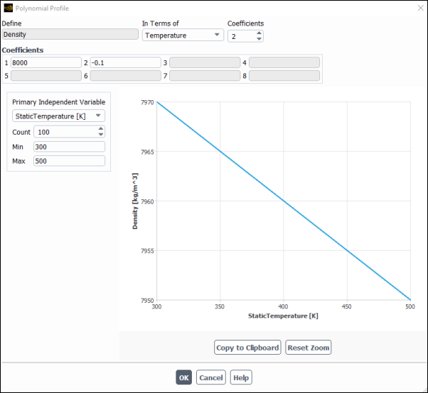
  1. Set Coefficients to 2.
  2. In the Coefficients group box, enter 8000 for 1 and -0.1 for 2.
    As shown in Figure 25.1: Solidification in Czochralski Model, the density of the material is defined by a polynomial function: .
  3. Click OK to close the Polynomial Profile dialog box.
4. In the Question dialog box, click Yes to overwrite air and add the new material (liquid-metal) to the Fluent Fluid Materials drop-down list.
5. Enter 680 for Cp (Specific Heat).
6. Enter 30 for Thermal Conductivity.
7. Enter 0.00553 for Viscosity.
8. Enter 100000 for Pure Solvent Melting Heat.
  Scroll down the group box to find Pure Solvent Melting Heat and the properties that follow.
  Note that for solidification to occur, Pure Solvent Melting Heat must be set to a positive non-zero value.
9. Enter 1150 for Solidus Temperature.
10. Enter 1150 for Liquidus Temperature.
11. Click Change/Create and close the Create/Edit Materials dialog box.

25.4.6. Setting the Cell Zone Conditions

Set the cell zone conditions for the fluid (fluid).
Setup → Cell Zone Conditions → Fluid → fluid Edit...
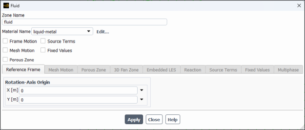
1. Ensure liquid-metal is selected from the Material Name drop-down list.
2. Click Apply and close the Fluid dialog box.

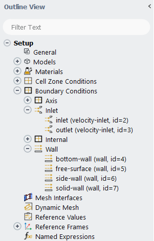
25.4.7. Setting the Boundary Conditions

Set the boundary conditions for the inlet (inlet).
Setup → Boundary Conditions → Inlet → inlet Edit...
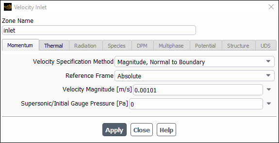
1. Enter 0.00101 for Velocity Magnitude.
2. Click the Thermal tab and enter 1300 for Temperature.
3. Click Apply and close the Velocity Inlet dialog box.
Set the boundary conditions for the outlet (outlet).
Setup → Boundary Conditions → Inlet → outlet Edit...
Here, the solid is pulled out with a specified velocity, so a velocity inlet boundary condition is used with a positive axial velocity component.
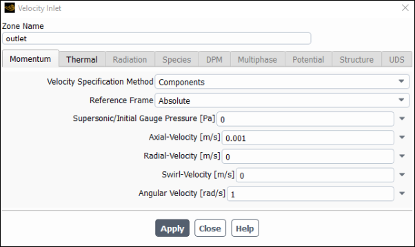
1. From the Velocity Specification Method drop-down list, select Components.
  The Velocity Inlet dialog box will change to show related inputs.
2. Enter 0.001 for Axial-Velocity.
3. Enter 1 for Angular Velocity.
4. Click the Thermal tab and enter 500 for Temperature.
5. Click Apply and close the Velocity Inlet dialog box.
Set the boundary conditions for the bottom wall (bottom-wall).
Setup → Boundary Conditions → Wall → bottom-wall Edit...
1. Click the Thermal tab.
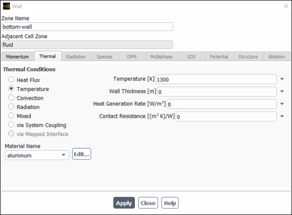
  1. Select Temperature in the Thermal Conditions group box.
  2. Enter 1300 for Temperature.
2. Click Apply and close the Wall dialog box.
Set the boundary conditions for the free surface (free-surface).
Setup → Boundary Conditions → Wall → free-surface Edit...
The specified shear and Marangoni stress boundary conditions are useful in modeling situations in which the shear stress (rather than the motion of the fluid) is known. A free surface condition is an example of such a situation. In this case, the convection is driven by the Marangoni stress and the shear stress is dependent on the surface tension, which is a function of temperature.
1. Select Marangoni Stress in the Shear Condition group box.
  The Marangoni Stress condition allows you to specify the gradient of the surface tension with respect to temperature at a wall boundary.
2. Enter -0.00036 for Surface Tension Gradient.
3. Click the Thermal tab to specify the thermal conditions.
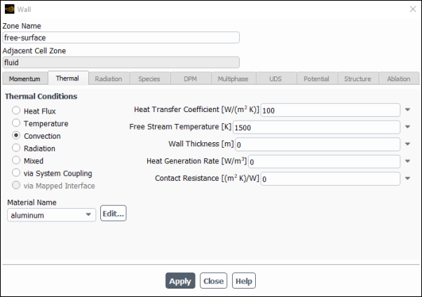
  1. Select Convection from the Thermal Conditions group box.
  2. Enter 100 for Heat Transfer Coefficient.
  3. Enter 1500 for Free Stream Temperature.
4. Click Apply and close the Wall dialog box.
Set the boundary conditions for the side wall (side-wall).
Setup → Boundary Conditions → Wall → side-wall Edit...
1. Click the Thermal tab.
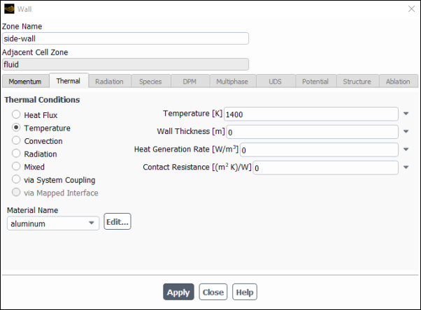
  1. Select Temperature from the Thermal Conditions group box.
  2. Enter 1400 for the Temperature.
2. Click Apply and close the Wall dialog box.
Set the boundary conditions for the solid wall (solid-wall).
Setup → Boundary Conditions → Wall → solid-wall Edit...
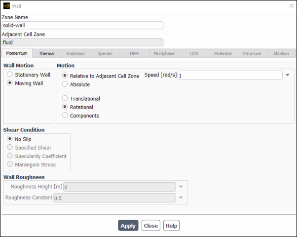
1. From the Wall Motion group box, select Moving Wall.
  The Wall dialog box is expanded to show additional parameters.
2. in the Motion group box, in the lower box, select Rotational.
  The Wall dialog box is changed to show the rotational speed.
3. Enter 1.0 for Speed.
4. Click the Thermal tab to specify the thermal conditions.
  1. Select Temperature from the Thermal Conditions selection list.
  2. Enter 500 for Temperature.
5. Click Apply and close the Wall dialog box.

25.4.8. Solution: Steady Conduction

In this step, you will specify the discretization schemes to be used and temporarily disable the calculation of the flow and swirl velocity equations, so that only conduction is calculated. This steady-state solution will be used as the initial condition for the time-dependent fluid flow and heat transfer calculation.

Set the solution parameters.
Solution → Solution → Methods...
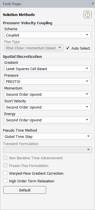
1. Select Coupled from the Scheme drop-down list in the Pressure-Velocity Coupling group box.
2. Select PRESTO! from the Pressure drop-down list in the Spatial Discretization group box.
  The PRESTO! scheme is well suited for rotating flows with steep pressure gradients.
3. Retain the default selection of Second Order Upwind from the Momentum, Swirl Velocity, and Energy drop-down lists.
4. Select Global Time Step from the Pseudo Time Method drop-down list.
  This Pseudo Time Method enables an algorithm in the coupled pressure-based solver that effectively adds an unsteady term to the solution equations, in order to improve stability and convergence behavior. The use of this option is recommended for general fluid flow problems.
Enable the calculation for energy.
Solution → Controls → Equations...
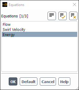
1. Deselect Flow and Swirl Velocity from the Equations selection list to disable the calculation of flow and swirl velocity equations.
2. Click OK to close the Equations dialog box.
Confirm the Relaxation Factors.
Solution → Controls → Controls...

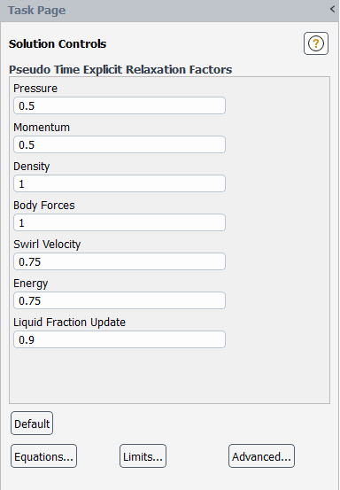
Retain the default values.
Enable the plotting of residuals during the calculation.
Solution → Reports → Residuals...
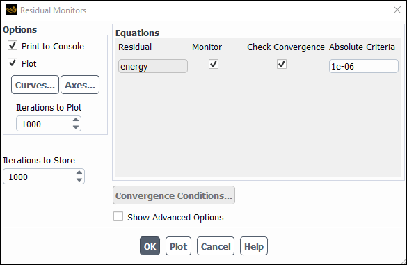
1. Ensure Plot is enabled in the Options group box.
2. Click OK to accept the remaining default settings and close the Residual Monitors dialog box.
Initialize the solution.
Solution → Initialization
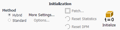
1. Retain the Method at the default of Hybrid in the Initialization group.
  For flows in complex topologies, hybrid initialization will provide better initial velocity and pressure field than standard initialization. This in general will help in improving the convergence behavior of the solver.
2. Click Initialize.
Define a custom field function for the swirl pull velocity.
Parameters & Customization → Custom Field Functions New...
In this step, you will define a field function to be used to patch a variable value for the swirl pull velocity in the next step. The swirl pull velocity is equal to , where is the angular velocity, and is the radial coordinate. Since = 1 rad/s, you can simplify the equation to simply . In this example, the value of is included for demonstration purposes.
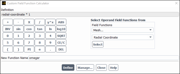
1. From the Field Functions drop-down lists, select Mesh... and Radial Coordinate.
2. Click the Select button to add radial-coordinate in the Definition field.
  If you make a mistake, click the DEL button on the calculator pad to delete the last item you added to the function definition.
3. Click the button on the calculator pad.
4. Click the 1 button.
5. Enter omegar for New Function Name.
6. Click Define.
  The omegar item appears under the Parameters & Customization/Parameters tree branch.
  Note: To check the function definition or delete the custom field function, click Manage.... Then in the Field Function Definitions dialog box, from the Field Functions selection list, select omegar to view the function definition.
7. Close the Custom Field Function Calculator dialog box.
Patch the pull velocities.
Solution → Initialization → Patch...
As noted earlier, you will patch values for the pull velocities, rather than having Ansys Fluent compute them. Since the radial pull velocity is zero, you will patch just the axial and swirl pull velocities.
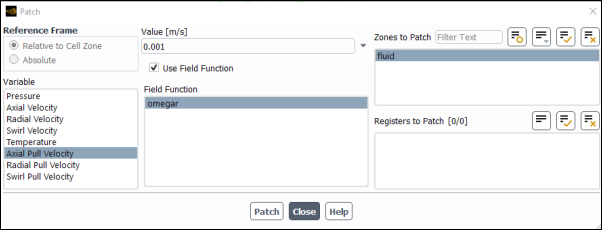
1. From the Variable selection list, select Axial Pull Velocity.
2. Enter 0.001 for Value.
3. From the Zones to Patch selection list, select fluid.
4. Click Patch.
  You have just patched the axial pull velocity. Next you will patch the swirl pull velocity.
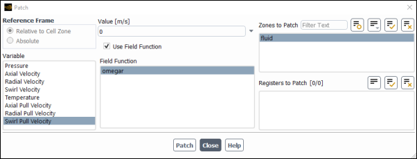
5. From the Variable selection list, select Swirl Pull Velocity.
  Scroll down the list to find Swirl Pull Velocity.
6. Enable the Use Field Function option.
7. Select omegar from the Field Function selection list.
8. Ensure that fluid is selected from the Zones to Patch selection list.
9. Click Patch and close the Patch dialog box.
Save the initial case and data files (solid0.cas.h5 and solid0.dat.h5).
File → Write → Case & Data...
Start the calculation by requesting 20 iterations.
Solution → Run Calculation → Run Calculation...
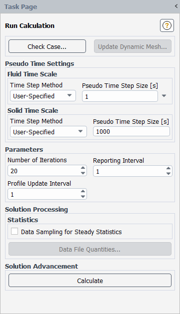
1. In the Run Calculation task page, select User-Specified for the Time Step Method in both the Fluid Time Scale and the Solid Time Scale group boxes.
2. Retain the default values of 1 s and 1000 s for the Pseudo Time Step Size in the Fluid Time Scale and the Solid Time Scale group boxes, respectively.
3. Enter 20 for Number of Iterations.
4. Click Calculate.
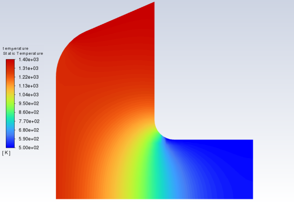
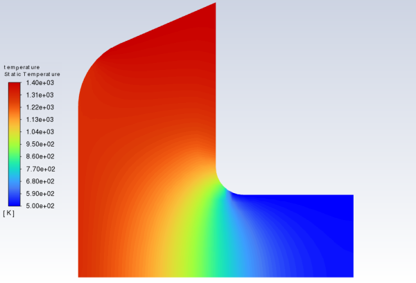
Create and display the definition of filled temperature contours (Figure 25.3: Contours of Temperature for the Steady Conduction Solution).
Results → Graphics → Contours → New...
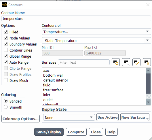
1. Enter temperature for Contour Name.
2. Enable the Filled option in the Options group box.
3. Select Banded in the Coloring group box.
4. Select Temperature... and Static Temperature from the Contours of drop-down lists.
5. Click Save/Display (Figure 25.3: Contours of Temperature for the Steady Conduction Solution) and close the Contours dialog box.
  The temperature contour definition appear under the Results/Graphics/Contours tree branch.
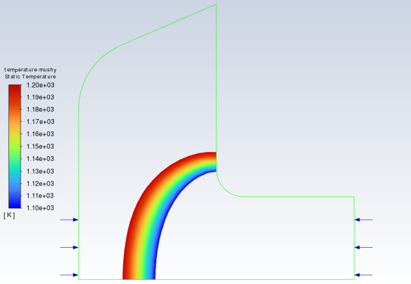
  Figure 25.3: Contours of Temperature for the Steady Conduction Solution
Display filled contours of temperature to determine the thickness of mushy zone.
Results → Graphics → Contours → New...
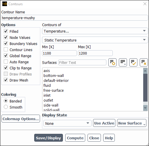
1. Enter temperature-mushy for Contour Name.
2. Disable Auto Range in the Options group box.
  The Clip to Range option is automatically enabled.
3. Enter 1100 for Min and 1200 for Max.
4. Select Banded in the Coloring group box.
5. Enable Draw Mesh in the Options group box.
6. Deselect default-interior from the Surfaces selection list and close the Mesh Display dialog box.
7. Click Save/Display (See Figure 25.4: Contours of Temperature (Mushy Zone) for the Steady Conduction Solution) and close the Contours dialog box.
Figure 25.4: Contours of Temperature (Mushy Zone) for the Steady Conduction Solution
Save the case and data files for the steady conduction solution (solid.cas.h5 and solid.dat.h5).
File → Write → Case & Data...

25.4.9. Solution: Transient Flow and Heat Transfer

In this step, you will turn on time dependence and include the flow and swirl velocity equations in the calculation. You will then solve the transient problem using the steady conduction solution as the initial condition.

Enable a time-dependent solution by selecting Transient from the Time list.
Setup → General
Set the solution parameters.
Solution → Solution → Methods...
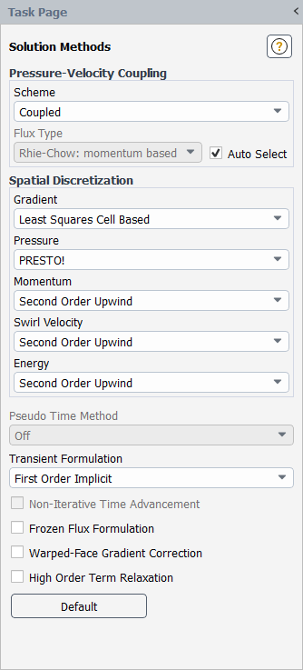
1. Retain the default selection of First Order Implicit from the Transient Formulation drop-down list.
2. Ensure that PRESTO! is selected from the Pressure drop-down list in the Spatial Discretization group box.
Enable calculations for flow and swirl velocity.
Solution → Controls → Equations...
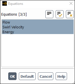
1. Select Flow and Swirl Velocity and ensure that Energy is selected from the Equations selection list.
  Now all three items in the Equations selection list will be selected.
2. Click OK to close the Equations dialog box.
Set the Under-Relaxation Factors.
Solution → Controls → Controls...
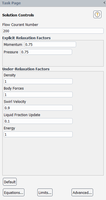
1. Enter 0.1 for Liquid Fraction Update.
2. Retain the default values for other Under-Relaxation Factors.
Save the initial case and data files (solid01.cas.h5 and solid01.dat.h5).
File → Write → Case & Data...
Run the calculation for 2 time steps.
Solution → Run Calculation → Run Calculation...
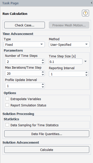
1. Enter 0.1s for Time Step Size.
2. Set the Number of Time Steps to 2.
3. Retain the default value of 20 for Max Iterations/Time Step.
4. Click Calculate.
Display filled contours of the temperature after 0.2 seconds using the temperature contours definition that you created earlier.
Results → Graphics → Contours → temperature Display
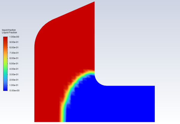
Figure 25.5: Contours of Temperature at t=0.2 s
Create and display the definition of liquid fraction contours by modifying the stream-function contour definition (Figure 25.6: Contours of Liquid Fraction at t=0.2 s).
Results → Graphics → Contours → New...
1. Enter liquid-fraction for Contour Name.
2. Enable Filled in the Options group box.
3. Enable Auto Range in the Options group box.
4. Select Solidification/Melting... and Liquid Fraction from the Contours of drop-down lists.
5. Click Save/Display and close the Contours dialog box.
Figure 25.6: Contours of Liquid Fraction at t=0.2 s

The liquid fraction contours show the current position of the melt front. Note that in Figure 25.6: Contours of Liquid Fraction at t=0.2 s, the mushy zone divides the liquid and solid regions roughly in half.
Continue the calculation for 48 additional time steps.
Solution → Run Calculation → Run Calculation...
1. Enter 48 for Number of Time Steps.
2. Click Calculate.
After a total of 50 time steps have been completed, the elapsed time will be 5 seconds.
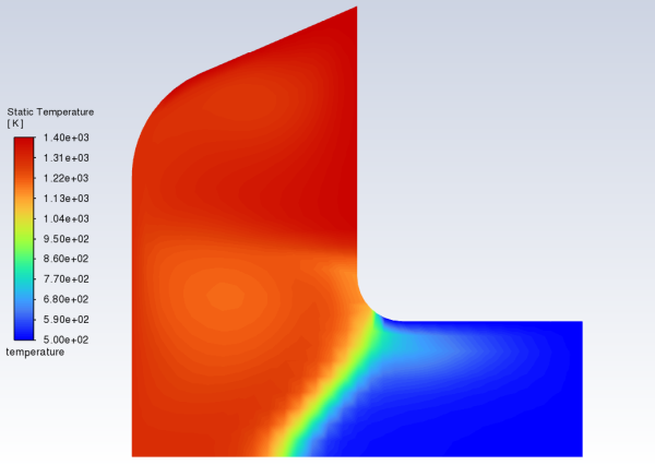
Display filled contours of the temperature after 5 seconds using the contour definition created earlier (Figure 25.7: Contours of Temperature at t=5 s).
Results → Graphics → Contours → temperature Display
Figure 25.7: Contours of Temperature at t=5 s

As shown in Figure 25.7: Contours of Temperature at t=5 s, the temperature contours are fairly uniform through the melt front and solid material. The distortion of the temperature field due to the recirculating liquid is also clearly evident.
In a continuous casting process, it is important to pull out the solidified material at the proper time. If the material is pulled out too soon, it will not have solidified (that is, it will still be in a mushy state). If it is pulled out too late, it solidifies in the casting pool and cannot be pulled out in the required shape. The optimal rate of pull can be determined from the contours of liquidus temperature and solidus temperature.
Display filled contours of liquid fraction (Figure 25.8: Contours of Liquid Fraction at t=5 s).
Results → Graphics → Contours → liquid-fraction Display
The introduction of liquid material at the left of the domain is balanced by the pulling of the solidified material from the right. After 5 seconds, the equilibrium position of the melt front is beginning to be established (Figure 25.8: Contours of Liquid Fraction at t=5 s).
Figure 25.8: Contours of Liquid Fraction at t=5 s
Save the case and data files for the solution at 5 seconds (solid5.cas.h5 and solid5.dat.h5).
File → Write → Case & Data...

25.5. Summary

In this tutorial, you studied the setup and solution for a fluid flow problem involving solidification for the Czochralski growth process.

The solidification model in Ansys Fluent can be used to model the continuous casting process where a solid material is continuously pulled out from the casting domain. In this tutorial, you patched a constant value and a custom field function for the pull velocities instead of computing them. This approach is used for cases where the pull velocity is not changing over the domain, as it is computationally less expensive than having Ansys Fluent compute the pull velocities during the calculation.

For more information about the solidification/melting model, see the Fluent User's Guide.