Chapter 24: Using the Eulerian Multiphase Model

This tutorial is divided into the following sections:

24.1. Introduction

This tutorial examines a turbulent two-phase flow consisting of air sparged into a water-filled mixing lab reactor. You will use the Eulerian multiphase model to simulate the mixing tank processes since the air and water phases are not in equilibrium throughout the simulation.

This tutorial demonstrates how to do the following:

Set up a multiphase flow simulation involving air and water.
Use multiple frames of reference.
Use a degassing outlet boundary condition to enable only air, but not water, to escape from the boundary.
Calculate a solution using the multiphase coupled solver with the Eulerian model.
Display the solution results.
Calculate torque and power requirements.

24.2. Prerequisites

This tutorial is written with the assumption that you have completed the introductory tutorials found in this manual and that you are familiar with the Ansys Fluent outline view and ribbon structure. Some steps in the setup and solution procedure will not be shown explicitly.

24.3. Problem Description

The problem to be modeled in this tutorial is shown schematically in Figure 24.1: Problem Schematic.

Figure 24.1: Problem Schematic

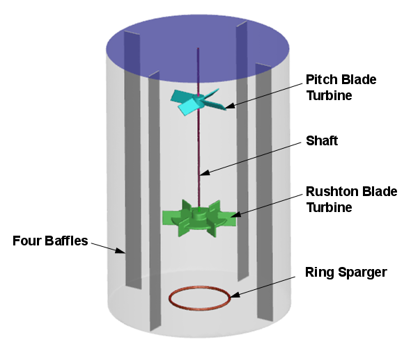
The geometry consists of a mixing vessel, four baffles along the vessel wall, a ring sparger, a pitch blade turbine, a Rushton blade turbine, and a rotating vertical shaft. There is no water flow into or out of the vessel. Air is injected into the tank at the bottom through the ring sparger at a speed of 0.05 m/s. Small inlet holes in the sparger ring are ignored, and the air inlet is modeled as a uniform circular strip. The air mixes with water, producing small bubbles. The Rushton blade turbine agitates the air-water mixture, evenly distributing the air bubbles. The pitch blade turbine performs dispersion and pumping operations. Both impellers rotate at 450 rpm in the counterclockwise direction about the Z axis (as viewed from the top). Dispersed gas bubbles can escape through the top water surface, which is open to the ambient air. This model can be used as a reasonable representation of the initial conditions in a real mixing tank.

24.4. Setup and Solution

The following sections describe the setup and solution steps for this tutorial:

24.4.1. Preparation

To prepare for running this tutorial:

Download the mixing_tank.zip file here .
Unzip mixing_tank.zip to your working directory.
The mesh file mixing_tank.msh.h5 can be found in the folder.
Use the Fluent Launcher to start Ansys Fluent.
Select Solution in the top-left selection list to start Fluent in Solution Mode.
Select 3D under Dimension.
Enable Double Precision under Options.
Set Solver Processes to 4 under Parallel (Local Machine).

24.4.2. Mesh

Read the mesh file mixing_tank.msh.h5.
File → Read → Mesh...
As Fluent reads the mesh file, it will report the progress in the console.
A warning message will be displayed that the degassing boundary condition type is not compatible with currently enabled models. You will resolve this issue when you enable the Eulerian multiphase model in a subsequent step.
Click OK and close the Information dialog box.
Check the mesh.
Domain → Mesh → Check → Perform Mesh Check
Fluent will perform various checks on the mesh and will report the progress in the console. Make sure that the reported minimum volume is a positive number.
Display the mesh.
Domain → Mesh → Display...
1. In the Options group box, enable Faces and Edges.
2. In the Surfaces selection list, select gas-inlet, wall_liquid_level and Wall (to select all walls), deselect fluid-tank_body.
3. Click Display and close the Mesh Display dialog box.
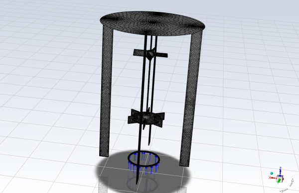
Examine the mesh (Figure 24.2: Mesh Display of the Mixing Tank).
Note: You can use the right mouse button to check which zone number corresponds to each boundary. If you click the right mouse button on one of the boundaries in the graphics window, its zone number, name, and type will be printed in the Ansys Fluent console. This feature is especially useful when you have several zones of the same type and you want to distinguish between them quickly.
Figure 24.2: Mesh Display of the Mixing Tank

24.4.3. Solver Settings

Related video that demonstrates steps for setting up, solving, and postprocessing the solution results for a two-phase turbulent flow within a mixing tank:

24.4.4. Models

Enable the Eulerian multiphase model.
Since you will use the default settings for the Eulerian model, you can enable it directly from the tree by right-clicking the Multiphase node and choosing Eulerian from the context menu.
Setup → Models → Multiphase Edit...
1. Select Eulerian under Model. Click Apply and close the Multiphase Model dialog box.
Click OK to close the Information dialog box.
Enabling the Eulerian multiphase model will also automatically enable the operating density parameters. You can verify this in the Operating Conditions dialog box.
Verify the operating density.
Physics → Solver → Operating Conditions...
1. Ensure that minimum-phase-averaged is selected from the Operating Density Method drop-down list.
2. Click OK to close the Operating Conditions dialog box.
Enable the k-ω turbulence model with standard wall functions.
Physics → Models → Viscous...
1. Retain the default k-omega (2 eqn) model in the Model group box.
2. Retain SST in the k-omega Model group box.
3. In the Turbulence Multiphase Model group box, select Dispersed.
  The dispersed turbulence model is suitable for cases when the dispersed phase is dilute. The model assumes that turbulence in the primary phase is dominant, while the turbulent quantities of the secondary phase can be obtained from the mean characteristics of the primary phase.
4. Click OK to close the Viscous Model dialog box.

24.4.5. Materials

The default properties for water defined in Ansys Fluent are suitable for this problem. In this step, you will make sure that this material is available for selecting in future steps.

Add water to the list of fluid materials by copying it from the Ansys Fluent materials database.
Setup → Materials → Fluid → air
1. Click Fluent Database... in the Create/Edit Materials dialog box to open the Fluent Database Materials dialog box.
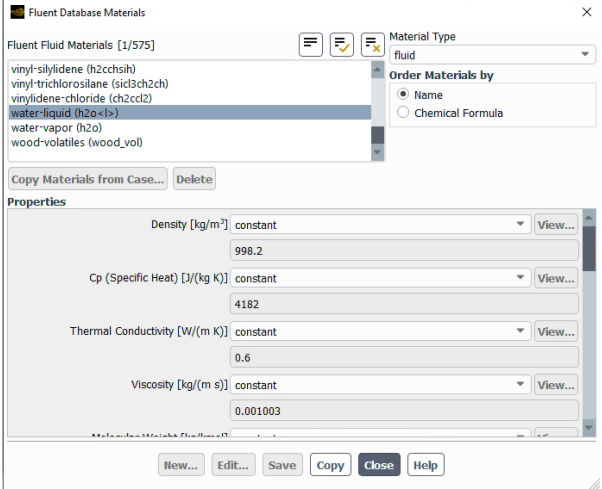
  1. Select water-liquid (h2o<l>) in the Fluent Fluid Materials selection list.
    Scroll down the list to find water-liquid (h2o<l>). Selecting this item will display the default properties in the dialog box.
  2. Click Copy and close the Fluent Database Materials dialog box.
  The Create/Edit Materials dialog box will now display the copied properties for water-liquid.
2. Click Change/Create and close the Create/Edit Materials dialog box.

24.4.6. Phases

In the following steps you will define the liquid water and air phases that flow in the mixing tank.

Setup → Models → Multiphase Edit...

In the Phases tab of the Multiphase Model dialog box, specify liquid water as the primary phase.
1. In the Phases selection list, select phase-1 – Primary Phase.
2. Enter water for Name.
3. Select water-liquid from the Phase Material drop-down list.
4. Click Apply.
Specify air as the secondary phase.
1. In the Phases selection list, select phase-2 – Secondary Phase.
2. Enter air for Name.
3. Retain the default selection of air from the Phase Material drop-down list.
4. Enter 0.0015 m for Diameter.
  The diameter of the air bubbles that are formed when the air is injected into the tank depends on the diameter of the inlet holes in the real reactor, which is 1 mm in this example.
5. Click Apply.
Define the interphase interactions formulations to be used.
1. Open the Phase Interaction tab.
2. In the Forces tab, select grace from the Coefficient drop-down list (Drag Coefficient group box).
  The Grace model is suitable for liquid-gas mixtures with low gas density and bubble sizes of 1-2 mm.
  Click OK to close the Grace Swarm Correction dialog box.
  Click OK to close the Information dialog box.
3. For Surface Tension Coefficients (Force Setup group box), select constant from the drop-down list and enter 0.073.
4. Click Apply and close the Multiphase Model dialog box.

24.4.7. Cell Zone Conditions

The mesh has three fluid cell zones: fluid_mrf_1-1 and fluid_mrf_2-0 are zones associated with the Rushton blade turbine and pitch blade turbine, respectively, and fluid_tank-2 represents the rest of the tank. In this section, you will use multiple reference frames to define boundary conditions for the cell zones that contain rotating components. Moving reference frames enable you to model the flow around rotating parts as steady-state with respect to the moving frames.

Physics → Zones → Cell Zones

Tip: To visually confirm the location of a cell or boundary zone, you can display it by right-clicking it in the tree and selecting either Display or Add to Graphics. Conversely, if you click a cell or boundary mesh in the graphics window, the selected item will be highlighted in the tree. You can use Ctrl or Shift to select multiple zones.

Set up the cell zone conditions for the fluid zone associated with the Rushton blade turbine (fluid_mrf_1-1).
Setup → Cell Zone Conditions → Fluid → fluid_mrf_1-1 Edit...
1. In the Fluid dialog box, enter rbt-zone for Zone Name.
  This name is more descriptive for the zone than fluid_mrf_1-1.
2. Select Frame Motion.
3. Retain the default values of (0, 0, 1) for X, Y, and Z in the Rotation-Axis Direction group box.
4. Enter 450 rev/min for Speed [rev/min] in the Rotational Velocity group box.
5. Click Apply and close the Fluid dialog box.
In a similar manner, set up the cell zone conditions for the fluid zone associated with the pitch blade turbine (fluid_mrf_2-0).
Setup → Cell Zone Conditions → Fluid → fluid_mrf_2-0 Edit...
1. In the Fluid dialog box, enter pbt-zone for Zone Name.
2. Select Frame Motion.
3. Retain the default values of (0, 0, 1) for X, Y, and Z in the Rotation-Axis Direction group box.
4. Enter 450 rev/min for Speed [rev/min] in the Rotational Velocity group box.
5. Click Apply and close the Fluid dialog box.
Retain the default settings for fluid_tank-2, which is stationary in the absolute reference frame.

24.4.8. Boundary Conditions

You will now define the conditions on the boundaries of the domain. Since each wall uses the same reference frame as the cell zone within which they are located, all walls will use the default stationary wall condition. A stationary wall condition implies that the wall is stationary with respect to the adjacent cell zone. Therefore, in the case of a rotating reference frame, a stationary wall is actually rotating with respect to the absolute reference frame.

The degassing boundary condition at the top of the fluid was created in a meshing application. At the degassing outlet, only gas phase can leave the domain. The degassing boundary condition became active after you enabled the Eulerian multiphase model in Fluent. No input is required for this type of boundary condition. For this problem, you only need to set the boundary conditions for the velocity inlet. Since this is a multiphase model, you will set the conditions that are specific to the primary and secondary phases.

Set the boundary conditions at the inlet (gas-inlet) for the primary phase (water).
Setup → Boundary Conditions → Inlet → gas-inlet → water Edit...
Since this is a dispersed turbulent flow, only turbulence must be defined for the water phase.
1. In the Turbulence group box, select Intensity and Hydraulic Diameter as the turbulence Specification Method.
2. Enter 3% for Turbulent Intensity.
3. Enter 0.0254 m for Hydraulic Diameter.
4. Click Apply and close the Velocity Inlet dialog box.
Set the boundary conditions at the inlet (gas-inlet) for the secondary phase (air).
Setup → Boundary Conditions → Inlet → gas-inlet → air Edit...
1. Enter 0.05 m/s for Velocity Magnitude.
2. In the Multiphase tab, enter 1 for Volume Fraction.
  A value of unity implies that only air enters the inlet.
3. Click Apply and close the Velocity Inlet dialog box.

24.4.9. Solution

Specify the discretization schemes.

Solution → Solution → Methods...

In the Solution Methods task page, configure the following settings.

Group Box	Setting	Value
Pressure Velocity Coupling	Scheme	Coupled
N/A	Pseudo Time Method	Global Time Step
N/A	Warped-Face Gradient Correction	(Enabled)

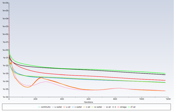
Ensure that Plot (plotting of residuals) is enabled during the calculation.
Solution → Reports → Residuals...
Initialize the solution.
Solution → Initialization → Initialize
Save the case file (mixing_tank.cas.h5).
File → Write → Case...
Start the calculation.
Solution → Run Calculation → Run Calculation...
1. Enter 1500 for Number of Iterations.
2. Retain the default selection of Automatic for the Time Step Method.
3. Retain the default value of 1 for Time Scale Factor.
4. Click Calculate.
Note: It may take significant time and computer resources to complete the problem calculation.
Figure 24.3: Residual History
After the solution has converged, save the case and data files (mixing_tank.cas.h5 and mixing_tank.dat.h5).
File → Write → Case & Data...

24.4.10. Postprocessing

Create iso-surfaces for y=0 and z=0.08.
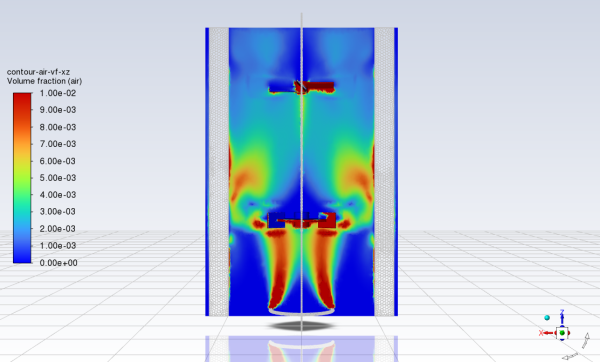
Display the distribution of air on the XZ plane (Figure 24.4: Contours of Air Volume Fraction on the XZ plane).
Results → Graphics → Contours → New...
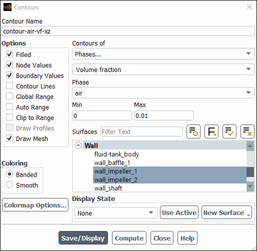
1. Enter contour-air-vf-xz for Contour Name.
2. From the Contours of drop-down lists, select Phases... and Volume Fraction.
3. From the Phase drop-down lists, select air.
4. In the Surfaces selection list, deselect all surfaces by clicking and then select y=0, wall_impeller_1, and wall_impeller_2.
5. In the Options group box, make sure that Filled is selected.
6. Disable Global Range, Auto Range, and Clip to Range.
7. Enter 0.01 for Max.
  The specified range will allow you to better view the volume fraction variation.
8. Select Draw Mesh to open the Mesh Display dialog box.
  1. In the Mesh Display dialog box, click next to the Surfaces filter to deselect all surfaces and then select wall_baffle_1, wall_sparger, and all walls whose names begin with wall_shaft.
  2. Enable Edges and disable Faces in the Options group box.
  3. Click Close to close the Mesh Display dialog box.
9. Ensure that Smooth is selected in the Coloring group box.
10. Click Save/Display and use the interactive triad to orient the view as shown in Figure 24.4: Contours of Air Volume Fraction on the XZ plane.
  Note: You may need to deselect Headlight and Lighting in the View ribbon tab (Display group).
  Figure 24.4: Contours of Air Volume Fraction on the XZ plane
  
  The contour map of the air volume fraction on the XZ plane shows how the air is agitated by impellers as it moves upward in the mixing tank. The shape of the Rushton blade turbine is forming cavities below the turbine.
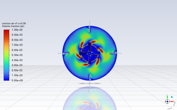
Display the distribution of air on the plane z=0.08 (Figure 24.5: Contours of Air Volume Fraction on the z=0.08 plane).
Results → Graphics → Contours → New...
1. Enter contour-air-vf-z=0.08 for Contour Name.
2. Set up the contour plot in a similar manner to step 1, except using the z=0.08 instead of y=0.
3. Click Save/Display and close the Contours dialog box.
4. In the View Tools toolbar, from the Set View drop-down list ( ), select the view from the positive Z axis ( ) to obtain the view shown in Figure 24.5: Contours of Air Volume Fraction on the z=0.08 plane.
  Figure 24.5: Contours of Air Volume Fraction on the z=0.08 plane
  
  Note that the air is collecting on the bottom surface of the Rushton blade turbine disk before its dispersed by the impeller’s blades.
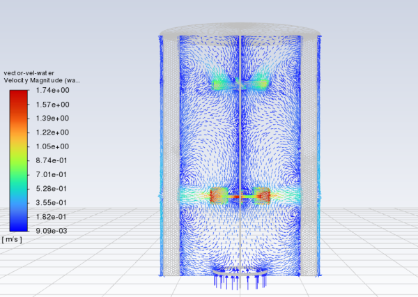
Display vectors of velocity magnitude for water on the XZ plane (Figure 24.6: Vectors of Water Velocity Magnitude on the XZ plane).
Results → Graphics → Vectors → New...
1. Enter vector-vel-water for Vector Name.
2. Disable Global Range.
3. Enable Draw Mesh and retain the default settings.
4. Select arrow from the Style drop-down list.
5. Select Velocity from the Vectors of drop-down list.
6. Select water from the Phase drop-down list.
  Since the Eulerian model solves individual momentum equations for each phase, you can choose the phase for which solution data is plotted.
7. From the Color by drop-down lists, select Velocity... and Velocity Magnitude.
8. Retain the selection of water from the Phase drop-down list.
9. In the Surfaces selection list, deselect all surfaces by clicking and then select y=0, wall_impeller_1, and wall_impeller_2.
10. Click Save/Display, close the Vectors dialog box, and use the interactive triad to orient the view as shown in Figure 24.6: Vectors of Water Velocity Magnitude on the XZ plane.
  Figure 24.6: Vectors of Water Velocity Magnitude on the XZ plane
  
  The vector plot of the water velocity shows that the water moves in a circular motion, creating a closed loop since it cannot escape the reactor.
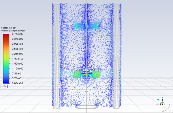
Display vectors of velocity magnitude for air on the XZ plane (Figure 24.7: Vectors of Air Velocity Magnitude on the XZ plane).
Results → Graphics → Vectors → New...
1. Enter vector-vel-air for Vector Name.
2. Enable Draw Mesh and retain the default settings.
3. Select arrow from the Style drop-down list.
4. Under Vectors of, select air from the Phase drop-down list.
5. Under Color by, select Velocity... and Velocity Magnitude.
6. In the Surfaces selection list, deselect all surfaces by clicking and then select y=0, wall_impeller_1, and wall_impeller_2.
7. Click Save/Display and close the Vectors dialog box.
  Figure 24.7: Vectors of Air Velocity Magnitude on the XZ plane
  
  The vector plot of the air velocity shows that the air moves upward all the way to the water surface, where it escapes. The baffle walls located on the sides of the tank prevent the undesirable vortex formation.
Calculate the torque about the shaft for the Rushton blade turbine.
Results → Reports → Forces...
1. From the Options group box, select Moments.
2. In the Moment Center group box, enter 0, 0, and 0 for X, Y, Z, respectively.
3. In the Moment Axis group box, enter 0, 0, and -1 for X, Y, Z, respectively.
4. From the Wall Zones selection list, deselect all zones by clicking and then select wall_impeller_1.
5. Click Print and close the Force Reports dialog box.
  Fluent reports the individual and net values of the pressure moment, viscous moment, total moment, pressure coefficient, viscous coefficient, and total coefficient about the specified center in the console.
  The power requirement is simply the required torque (0.03767 N m) multiplied by the rotational speed (450 rpm = 47.12 rad/s): 0.03767 N m * 47.1 rad/s = 1.77 W.
  Note that this value does not account for any mechanical losses, motor efficiencies, and so on.
Save the case file (mixing_tank.cas.h5).
File → Write → Case...

24.5. Summary

This tutorial demonstrated how to set up and solve a turbulent multiphase flow in the mixing tank using the Eulerian multiphase model. You learned how to set degassing boundary conditions and boundary conditions for primary and secondary phases. After completing the simulation, you displayed the results of your calculation and calculated the torque and power requirements. For more information about the Eulerian multiphase model, see the Fluent User's Guide.