Chapter 26: Using the Eulerian Granular Multiphase Model with Heat Transfer

This tutorial is divided into the following sections:

26.1. Introduction

This tutorial examines the flow of air and a granular solid phase consisting of glass beads in a hot gas fluidized bed, under uniform minimum fluidization conditions. The results obtained for the local wall-to-bed heat transfer coefficient in Ansys Fluent can be compared with analytical results [1].

This tutorial demonstrates how to do the following:

Use the Eulerian granular model.
Set boundary conditions for internal flow.
Compile a User-Defined Function (UDF) for the gas and solid phase thermal conductivities.
Calculate a solution using the pressure-based solver.

26.2. Prerequisites

This tutorial is written with the assumption that you have completed the introductory tutorials found in this manual and that you are familiar with the Ansys Fluent outline view and ribbon structure. Some steps in the setup and solution procedure will not be shown explicitly.

In order to complete the steps to compile the UDF, you will need to have a working C compiler installed on your machine.

26.3. Problem Description

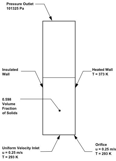
This problem considers a hot gas fluidized bed in which air flows upwards through the bottom of the domain and through an additional small orifice next to a heated wall. A uniformly fluidized bed is examined, which you can then compare with analytical results [1]. The geometry and data for the problem are shown in Figure 26.1: Problem Schematic.

Figure 26.1: Problem Schematic

26.4. Setup and Solution

The following sections describe the setup and solution steps for this tutorial:

26.4.1. Preparation

To prepare for running this tutorial:

Download the eulerian_granular_heat.zip file here .
Unzip eulerian_granular_heat.zip to your working directory.
The files fluid-bed.msh and conduct.c can be found in the folder.
Use the Fluent Launcher to start Ansys Fluent.
Select Solution in the top-left selection list to start Fluent in Solution Mode.
Select 2D under Dimension.
Enable Double Precision under Options.

Note: The double precision solver is recommended for modeling multiphase flow simulations.
Set Solver Processes to 1 under Parallel (Local Machine).

26.4.2. Mesh

Read the mesh file fluid-bed.msh.
File → Read → Mesh...
As Ansys Fluent reads the mesh file, it will report the progress in the console.
Check the mesh.
Domain → Mesh → Check → Perform Mesh Check
Ansys Fluent will perform various checks on the mesh and will report the progress in the console. Make sure that the reported minimum volume is a positive number.
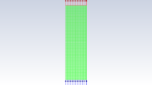
Examine the mesh (Figure 26.2: Mesh Display of the Fluidized Bed).
Note: You can use the right mouse button to check which zone number corresponds to each boundary. If you click the right mouse button on one of the boundaries in the graphics window, its zone number, name, and type will be printed in the Ansys Fluent console. This feature is especially useful when you have several zones of the same type and you want to distinguish between them quickly.
Figure 26.2: Mesh Display of the Fluidized Bed

26.4.3. Solver Settings

Enable the pressure-based transient solver.
Setup → General
1. Retain the default selection of Pressure-Based from the Type list.
  The pressure-based solver must be used for multiphase calculations.
2. Select Transient from the Time list.
3. Enable Gravity.
4. Enter -9.81 m/s² for the Gravitational Acceleration in the Y direction.

26.4.4. Models

Enable the Eulerian multiphase model for two phases.
You will use the default settings for the Eulerian model, so you can enable it directly from the tree by right-clicking the Multiphase node and choosing Eulerian from the context menu.
Setup → Models → Multiphase Eulerian
Enable heat transfer by enabling the energy equation.
Setup → Models → Energy On
An Information dialog box appears reminding you to confirm the property values. Click OK in the Information dialog box to continue.
Enable the laminar viscous model.
The decision to use the laminar model should be based on the Stokes number for the particles suspended in the fluid flow.
Setup → Models → Viscous Model → Laminar

26.4.5. UDF

Compile the user-defined function, conduct.c, that will be used to define the thermal conductivity for the gas and solid phases.
User Defined → User Defined → Functions → Compiled...
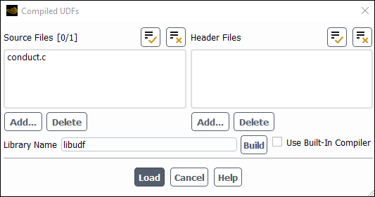
1. Click the Add... button below the Source Files option to open the Select File dialog box.
2. Select the file conduct.c and click OK in the Select File dialog box.
3. Click Build.
  Ansys Fluent will create a libudf folder and compile the UDF. Also, a Warning dialog box will open asking you to make sure that UDF source file and case/data files are in the same folder.
4. Click OK to close the Warning dialog box.
5. Click Load to load the UDF.

26.4.6. Materials

Modify the properties for air, which will be used for the primary phase.
Setup → Materials → air → Create/Edit...
The properties used for air are modified to match data used by Kuipers et al. [1]
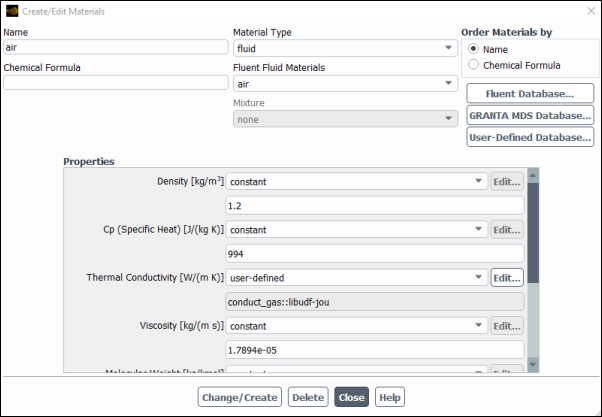
1. Enter 1.2 kg/m³ for Density.
2. Enter 994 J/kg-K for Cp.
3. Select user-defined from the Thermal Conductivity drop-down list to open the User Defined Functions dialog box.
  1. Select conduct_gas::libudf from the available list.
  2. Click OK to close the User Defined Functions dialog box.
4. Click Change/Create and close the Materials dialog box..
Define a new fluid material for the granular phase (the glass beads).
Setup → Materials → air → Create/Edit...
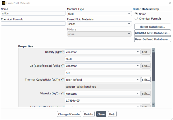
1. Enter solids for Name.
2. Enter 2660 kg/m³ for Density.
3. Enter 737 J/kg-K for Cp.
4. Retain the selection of user-defined from the Thermal Conductivity drop-down list.
5. Click the Edit... button to open the User Defined Functions dialog box.
  1. Select conduct_solid::libudf in the User Defined Functions dialog box and click OK.
    A Question dialog box will open asking if you want to overwrite air.
  2. Click No in the Question dialog box.
6. Click Change/Create and close the Materials dialog box.

26.4.7. Phases

You will now configure the phases.

Setup → Models → Multiphase Edit...

In the Phases tab of the Multiphase Model dialog box, define air as the primary phase.
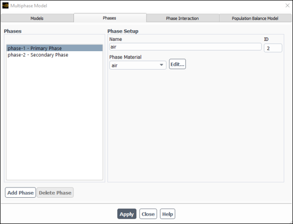
1. In the Phases selection list, select phase-1 – Primary Phase.
2. Enter air for Name.
3. Ensure that air is selected from the Phase Material drop-down list.
4. Click Apply.
  Important: When setting up your case, if you have made changes in the current tab, you should click the Apply button to make them effective before moving to the next tab. Otherwise, the relevant models may not be available in the other tabs, and your settings may be lost.
Define solids (glass beads) as the secondary phase.
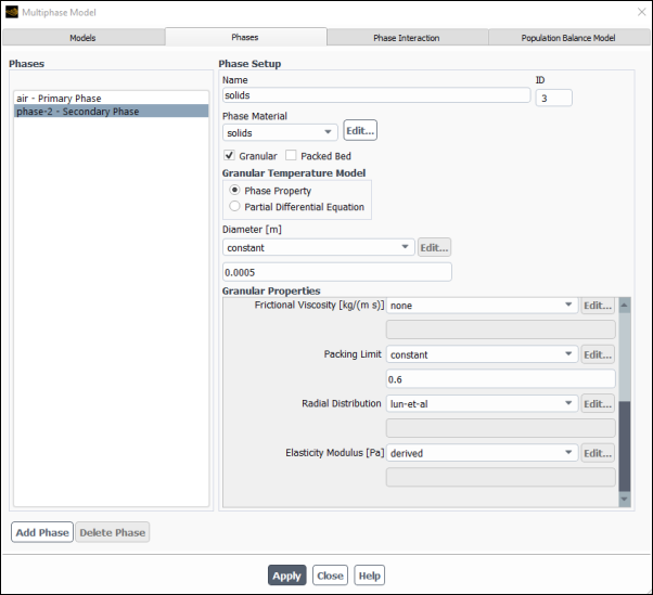
1. In the Phases selection list, select phase-2 – Secondary Phase.
2. Enter solids for Name.
3. Select solids from the Phase Material drop-down list.
4. Enable Granular.
5. Retain the default selection of Phase Property in the Granular Temperature Model group box.
6. Enter 0.0005 m for Diameter.
7. Select syamlal-obrien from the Granular Viscosity drop-down list.
8. Select lun-et-al from the Granular Bulk Viscosity drop-down list.
9. Select constant from the Granular Temperature drop-down list and enter 1e-05.
10. Enter 0.6 for the Packing Limit.
11. Click Apply.
In the Phases Interaction tab of the Multiphase Model dialog box, define the interphase interactions formulations to be used.
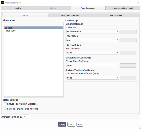
1. In the Forces tab, select syamlal-obrien from the Coefficient drop-down list (Drag Coefficient group box).
2. Click Apply.
3. Go to the Heat, Mass, Reactions tab.
4. In the Heat tab, select gunn from the Heat Transfer Coefficient drop-down list.
  The interphase heat exchange is simulated, using a drag coefficient, the default restitution coefficient for granular collisions of 0.9, and a heat transfer coefficient. Granular phase lift is not very relevant in this problem, and in fact is rarely used.
5. Click Apply.
6. In the Interfacial Area tab, select ia-symmetric from the Interfacial Area drop-down list.
  The default ia-particle method is best suited for typical dispersed flow applications with a volume fraction lower than 30%. In this analysis, the volume fraction of the secondary phase is relatively high (close to 60%). The ia-symmetric correlation is more accurate for such cases because it considers the volume fraction of both the primary and secondary phases in the interfacial area calculation.
7. Click Apply and close the Multiphase Model dialog box.

26.4.8. Boundary Conditions

For this problem, you need to set the boundary conditions for all boundaries.

Setup → Boundary Conditions

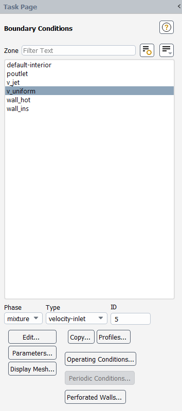
Set the boundary conditions for the lower velocity inlet (v_uniform) for the primary phase.
Setup → Boundary Conditions → v_uniform
For the Eulerian multiphase model, you will specify conditions at a velocity inlet that are specific to the primary and secondary phases.
1. Select air from the Phase drop-down list.
2. Click the Edit... button to open the Velocity Inlet dialog box.
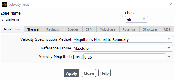
  1. Retain the default selection of Magnitude, Normal to Boundary from the Velocity Specification Method drop-down list.
  2. Enter 0.25 m/s for the Velocity Magnitude.
  3. Click the Thermal tab and enter 293 K for Temperature.
  4. Click Apply and close the Velocity Inlet dialog box.
3. 1. Select solids from the Phase drop-down list.
  2. Click the Edit... button to open the Velocity Inlet dialog box.
    
    Retain the default Velocity Specification Method and Reference Frame.
    Retain the default value of 0 m/s for the Velocity Magnitude.
    Click the Thermal tab and enter 293 K for Temperature.
    Click the Multiphase tab and retain the default value of 0 for Volume Fraction.
    Click Apply and close the Velocity Inlet dialog box.
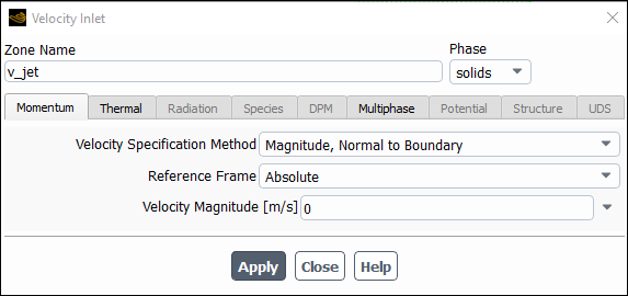
Set the boundary conditions for the orifice velocity inlet (v_jet) for the primary phase.
Setup → Boundary Conditions → v_jet
1. Select air from the Phase drop-down list.
2. Click the Edit... button to open the Velocity Inlet dialog box.
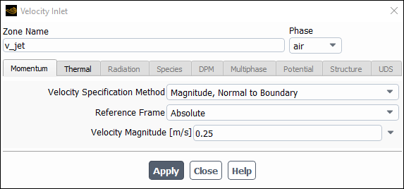
  1. Retain the default Velocity Specification Method and Reference Frame.
  2. Enter 0.25 m/s for the Velocity Magnitude.
    In order for a comparison with analytical results [1] to be meaningful, in this simulation you will use a uniform value for the air velocity equal to the minimum fluidization velocity at both inlets on the bottom of the bed.
  3. Click the Thermal tab and enter 293 K for Temperature.
  4. Click Apply and close the Velocity Inlet dialog box.
3. 1. Select solids from the Phase drop-down list.
  2. Click the Edit... button to open the Velocity Inlet dialog box.
    
    Retain the default Velocity Specification Method and Reference Frame.
    Retain the default value of 0 m/s for the Velocity Magnitude.
    Click the Thermal tab and enter 293 K for Temperature.
    Click the Multiphase tab and retain the default value of 0 for the Volume Fraction.
    Click Apply and close the Velocity Inlet dialog box.
Set the boundary conditions for the pressure outlet (poutlet) for the mixture phase.
Setup → Boundary Conditions → poutlet
For the Eulerian granular model, you will specify conditions at a pressure outlet for the mixture and for both phases.
The thermal conditions at the pressure outlet will be used only if flow enters the domain through this boundary. You can set them equal to the inlet values, as no flow reversal is expected at the pressure outlet. In general, however, it is important to set reasonable values for these downstream scalar values, in case flow reversal occurs at some point during the calculation.
1. Select mixture from the Phase drop-down list.
2. Click the Edit... button to open the Pressure Outlet dialog box.
  1. Retain the default value of 0 Pascal for Gauge Pressure.
  2. Click Apply and close the Pressure Outlet dialog box.
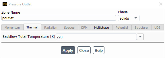
Set the boundary conditions for the pressure outlet (poutlet) for the primary phase.
Setup → Boundary Conditions → poutlet
1. Select air from the Phase drop-down list.
2. Click the Edit... button to open the Pressure Outlet dialog box.
  1. In the Thermal tab, enter 293 K for Backflow Total Temperature.
  2. Click Apply and close the Pressure Outlet dialog box.
3. 1. Select solids from the Phase drop-down list.
  2. Click the Edit... button to open the Pressure Outlet dialog box.
    
    In the Thermal tab, enter 293 K for the Backflow Total Temperature.
    In the Multiphase tab, retain default settings.
    Click Apply and close the Pressure Outlet dialog box.
Set the boundary conditions for the heated wall (wall_hot) for the mixture.
Setup → Boundary Conditions → wall_hot
For the heated wall, you will set thermal conditions for the mixture, and momentum conditions (zero shear) for both phases.
1. Select mixture from the Phase drop-down list.
2. Click the Edit... button to open the Wall dialog box.
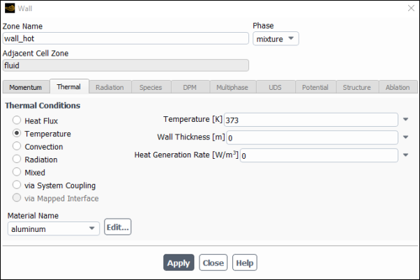
  1. In the Thermal tab, select Temperature from the Thermal Conditions list.
  2. Enter 373 K for Temperature.
  3. Click Apply and close the Wall dialog box.
Set the boundary conditions for the heated wall (wall_hot) for the primary phase.
Setup → Boundary Conditions → wall_hot
1. Select air from the Phase drop-down list.
2. Click the Edit... button to open the Wall dialog box.
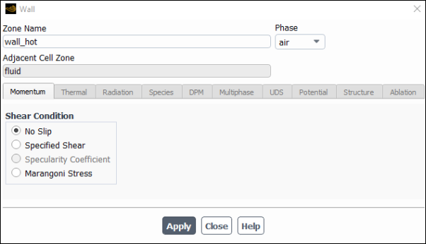
3. Retain the default No Slip condition and click Apply and close the Wall dialog box.
Set the boundary conditions for the adiabatic wall (wall_ins).
Setup → Boundary Conditions → wall_ins
For the adiabatic wall, retain the default thermal conditions for the mixture (zero heat flux), and the default momentum conditions (no slip) for both phases.

26.4.9. Solution

Select the second order implicit transient formulation and higher-order spatial discretization schemes.
Solution → Solution → Methods...
1. Modify the discretization methods in the Spacial Discretization group box.
  1. Select Second Order for Pressure and Second Order Upwind for Momentum.
  2. Select QUICK for Volume Fraction and Energy.
2. Select Second Order Implicit from the Transient Formulation drop-down list.
Set the solution parameters.
Solution → Controls → Controls...
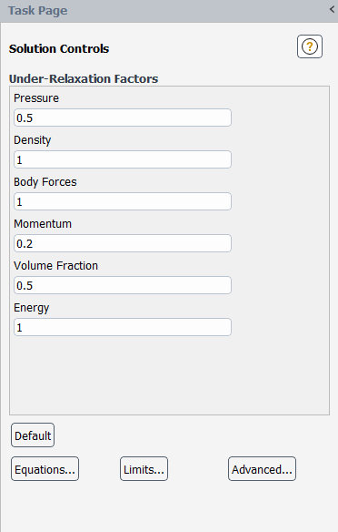
1. Enter 0.5 for Pressure.
2. Enter 0.2 for Momentum.
Ensure that the plotting of residuals is enabled during the calculation.
Solution → Reports → Residuals...
Define a custom field function for the heat transfer coefficient.
User Defined → Field Functions → Custom...
Initially, you will define functions for the mixture temperature, and thermal conductivity, then you will use these to define a function for the heat transfer coefficient.
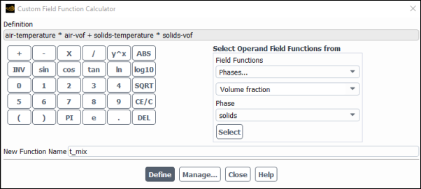
1. Define the function t_mix.
  1. Select Temperature... and Static Temperature from the Field Functions drop-down lists.
  2. Ensure that air is selected from the Phase drop-down list and click Select.
  3. Click the multiplication symbol in the calculator pad.
  4. Select Phases... and Volume fraction from the Field Functions drop-down list.
  5. Ensure that air is selected from the Phase drop-down list and click Select.
  6. Click the addition symbol in the calculator pad.
  7. Similarly, add the term solids-temperature * solids-vof.
  8. Enter t_mix for New Function Name.
  9. Click Define.
2. Define the function k_mix.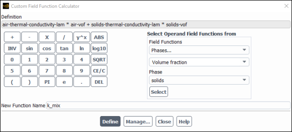
  1. Select Properties... and Thermal Conductivity from the Field Functions drop-down lists.
  2. Select air from the Phase drop-down list and click Select.
  3. Click the multiplication symbol in the calculator pad.
  4. Select Phases... and Volume fraction from the Field Functions drop-down lists.
  5. Ensure that air is selected from the Phase drop-down list and click Select.
  6. Click the addition symbol in the calculator pad.
  7. Similarly, add the term solids-thermal-conductivity-lam * solids-vof.
  8. Enter k_mix for New Function Name.
  9. Click Define.
3. Define the function ave_htc.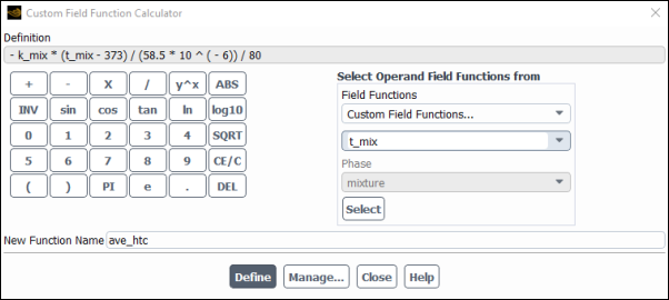
  1. Click the subtraction symbol in the calculator pad.
  2. From the Field Functions drop-down lists, select Custom Field Functions... and k_mix and click Select.
  3. Use the calculator pad and the Field Functions lists to complete the definition of the function.
  4. Enter ave_htc for New Function Name.
  5. Click Define and close the Custom Field Function Calculator dialog box.
Define the point surface in the cell next to the wall on the plane .
Domain → Surface → Create → Point...
1. Enter y=0.24 for New Surface Name.
2. Enter 0.28494 m for x and 0.24 m for y in the Coordinates group box.
3. Click Create and close the Point Surface dialog box.
Create a surface report definition for the heat transfer coefficient.
Solution → Reports → Definitions → New → Surface Report → Facet Average...
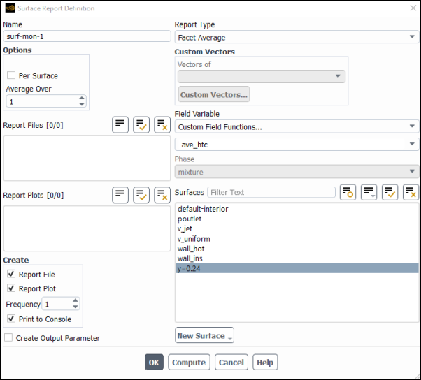
1. Enter surf-mon-1 for Name of the surface report definition.
2. In the Create group box, enable Report File, Report Plot and Print to Console.
3. Select Custom Field Functions... and ave_htc from the Field Variable drop-down lists.
4. Select y=0.24 from the Surfaces selection list.
5. Click OK to save the surface report definition settings and close the Surface Report Definition dialog box.
  surf-mon-1-rplot and surf-mon-1-rfile that are automatically generated by Fluent appear in the tree (under Solution/Monitors/Report Plots and Solution/Monitors/Report Files, respectively).
6. Rename the report output file.
  Solution → Monitors → Report Files → surf-mon-1-rfile Edit...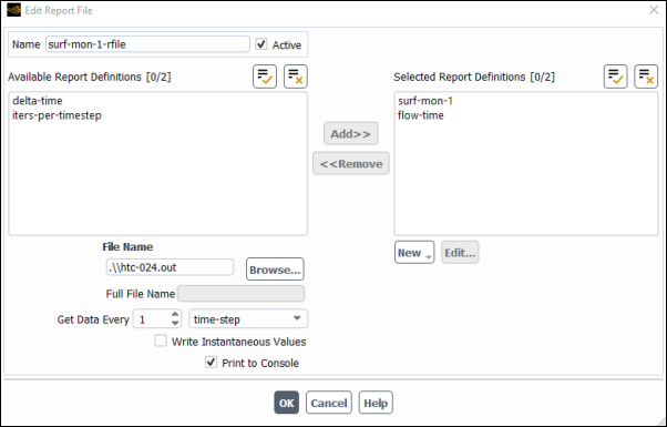
  1. Enter htc-024.out for Output File Base Name.
  2. Click OK to close the Edit Report File dialog box.
Define a cell register for the lower half of the fluidized bed.
Solution → Cell Registers New → Region...
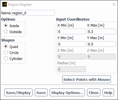
1. Enter 0.3 m for Xmax and 0.5 m for Ymax in the Input Coordinates group box.
2. Click Save and close the Region Register dialog box.
This register is used to patch the initial volume fraction of solids in the next step.
Initialize the solution.
Solution → Initialization → Options...
1. Select all-zones from the Compute from drop-down list.
2. Retain the default values and click Initialize.
Patch the initial volume fraction of solids in the lower half of the fluidized bed.
Solution → Initialization → Patch...
1. Select solids from the Phase drop-down list.
2. Select Volume Fraction from the Variable selection list.
3. Enter 0.598 for Value.
4. Select region_0 from the Registers to Patch selection list.
5. Click Patch and close the Patch dialog box.
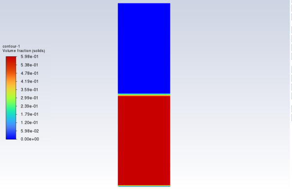
At this point, it is a good practice to display contours of the variable you just patched, to ensure that the desired field was obtained.
Display contours of Volume Fraction of solids (Figure 26.3: Initial Volume Fraction of Granular Phase (solids)).
Results → Graphics → Contours → New...
1. Enable Filled in the Options group box.
2. Select Phases... from the upper Contours of drop-down list.
3. Select solids from the Phase drop-down list.
4. Ensure that Volume fraction is selected from the lower Contours of drop-down list.
5. Click Save/Display and close the Contours dialog box.
Figure 26.3: Initial Volume Fraction of Granular Phase (solids)
Save the case file (fluid-bed.cas.h5).
File → Write → Case...
Start calculation.
Solution → Run Calculation → Run Calculation...
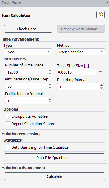
1. Set 0.00015 for Time Step Size.
2. Set 12000 for Number of Time Steps.
3. Enter 50 for Max Iterations/Time Step.
4. Click Calculate.
The plot of the value of the mixture-averaged heat transfer coefficient in the cell next to the heated wall versus time is in excellent agreement with results published for the same case [1].
Figure 26.4: Plot of Mixture-Averaged Heat Transfer Coefficient in the Cell Next to the Heated Wall Versus Time
Save the case and data files (fluid-bed.cas.h5 and fluid-bed.dat.h5).
File → Write → Case & Data...

26.4.10. Postprocessing

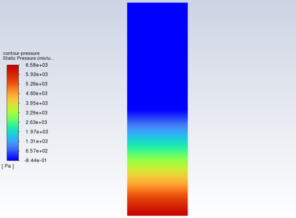
Display the pressure field in the fluidized bed (Figure 26.5: Contours of Static Pressure).
Results → Graphics → Contours → New...
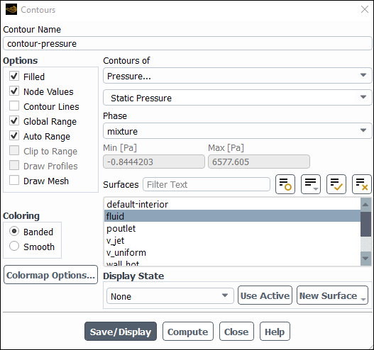
1. Enter contour-pressure for Contour Name.
2. Select Banded in the Coloring group box.
3. Select mixture from Phase drop-down list.
4. Select Pressure... and Static Pressure from the Contours of drop-down lists.
5. Click Save/Display and close the Contours dialog box.
  Figure 26.5: Contours of Static Pressure
  
  Note the build-up of static pressure in the granular phase.
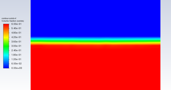
Display the volume fraction of solids (Figure 26.6: Contours of Volume Fraction of Solids).
Results → Graphics → Contours → New...
1. Enter contour-solid-vf for Contour Name.
2. Select Banded in the Coloring group box.
3. Select solids from the Phase drop-down list.
4. Select Phases... and Volume fraction from the Contours of drop-down lists.
5. Click Save/Display and close the Contours dialog box.
6. Zoom in to show the contours close to the region where the change in volume fraction is the greatest.
Note that the region occupied by the granular phase has expanded slightly, as a result of fluidization.
Figure 26.6: Contours of Volume Fraction of Solids
Save the case file (fluid-bed.cas.h5).
File → Write → Case...

26.5. Summary

This tutorial demonstrated how to set up and solve a granular multiphase problem with heat transfer, using the Eulerian model. You learned how to set boundary conditions for the mixture and both phases. The solution obtained is in excellent agreement with analytical results from Kuipers et al. [1].

26.6. References

J. A. M. Kuipers, W. Prins, and W. P. M. Van Swaaij "Numerical Calculation of Wall-to-Bed Heat Transfer Coefficients in Gas-Fluidized Beds", Department of Chemical Engineering, Twente University of Technology, in AIChE Journal, July 1992, Vol. 38, No. 7.