Chapter 21: Modeling Evaporating Liquid Spray

This tutorial is divided into the following sections:

21.1. Introduction

In this tutorial, the air-blast atomizer model in Ansys Fluent is used to predict the behavior of an evaporating methanol spray. Initially, the air flow is modeled without droplets. To predict the behavior of the spray, the discrete phase model is used, including a secondary model for breakup.

This tutorial demonstrates how to do the following:

Define a spray injection for an air-blast atomizer.
Calculate a solution using the discrete phase model in Ansys Fluent.

21.2. Prerequisites

This tutorial is written with the assumption that you have completed the introductory tutorials found in this manual and that you are familiar with the Ansys Fluent outline view and ribbon structure. Some steps in the setup and solution procedure will not be shown explicitly.

21.3. Problem Description

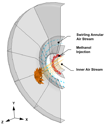
The geometry to be considered in this tutorial is shown in Figure 21.1: Problem Specification. Methanol is cooled to -10°C before being introduced into an air-blast atomizer. The atomizer contains an inner air stream surrounded by a swirling annular stream. To make use of the periodicity of the problem, only a 30° section of the atomizer will be modeled.

Figure 21.1: Problem Specification

21.4. Setup and Solution

The following sections describe the setup and solution steps for this tutorial:

21.4.1. Preparation

To prepare for running this tutorial:

Download the evaporate_liquid.zip file here .
Unzip evaporate_liquid.zip to your working directory.
The mesh file sector.msh.h5 can be found in the folder.
Use the Fluent Launcher to start Ansys Fluent.
Select Solution in the top-left selection list to start Fluent in Solution Mode.
Select 3D under Dimension.
Enable Double Precision under Options.
Set Solver Processes to 1 under Parallel (Local Machine).

21.4.2. Mesh

Read in the mesh file sector.msh.h5.
File → Read → Mesh...
Change the periodic type of periodic-a to rotational.
Setup → Boundary Conditions → Periodic → periodic-a Edit...
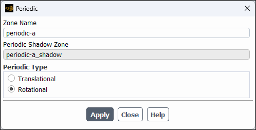
1. Select Rotational in the Periodic Type group box.
2. Click Apply and close the Periodic dialog box.
In a similar manner, change the periodic type of periodic-b to rotational.
Check the mesh.
Domain → Mesh → Check → Perform Mesh Check
Ansys Fluent will perform various checks on the mesh and report the progress in the console. Ensure that the reported minimum volume is a positive number.
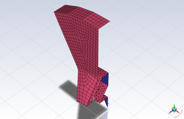
Display the mesh.
Domain → Mesh → Display...
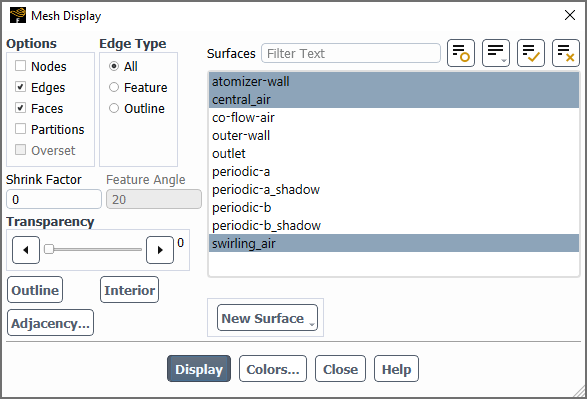
1. Ensure that Edges and Faces are enabled in the Options group box.
2. Select only atomizer-wall, central_air, and swirling_air from the Surfaces selection list.
  Tip: To deselect all surfaces click the far-right button at the top of the Surfaces selection list, and then select the desired surfaces from the Surfaces selection list.
3. Click the Colors... button to open the Mesh Colors dialog box.
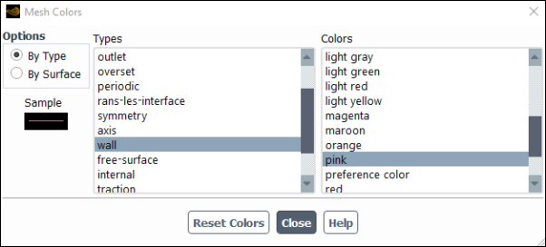
  1. Select wall from the Types selection list.
  2. Select pink from the Colors selection list.
  3. Close the Mesh Colors dialog box.
4. Click Display and close the Mesh Display dialog box.
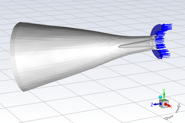
The graphics display will be updated to show the mesh. Zoom in with the mouse to obtain the view shown in Figure 21.2: Air-Blast Atomizer Mesh Display.
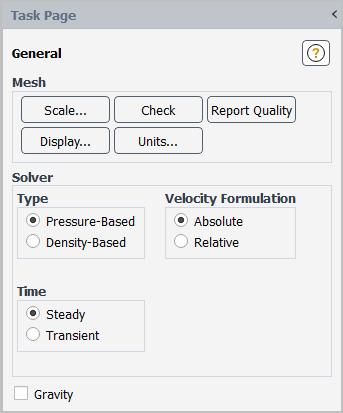
Figure 21.2: Air-Blast Atomizer Mesh Display

21.4.3. Solver

Retain the default solver settings of pressure-based steady-state solver in the General task page (Solver and Time group boxes).

Physics → Solver → General...

21.4.4. Models

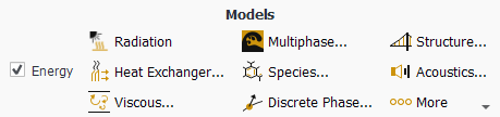
Enable heat transfer by enabling the energy equation.
Physics → Models → Energy
Enable the k-ω SST turbulence model.
Physics → Models → Viscous...
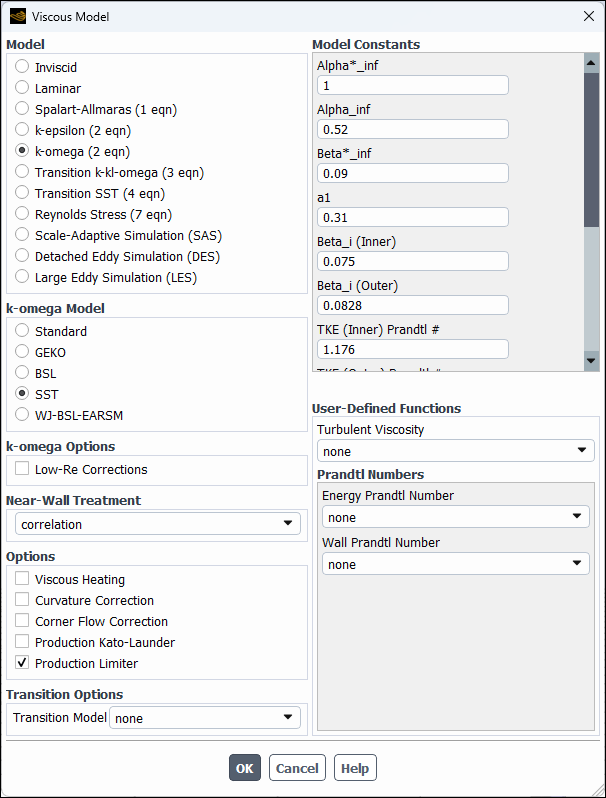
1. Retain the default selection of k-omega (2 eqn) in the Model list.
2. Retain the default selection of SST in the k-omega Model list.
3. Click OK to close the Viscous Model dialog box.
Enable chemical species transport and reaction.
Physics → Models → Species...
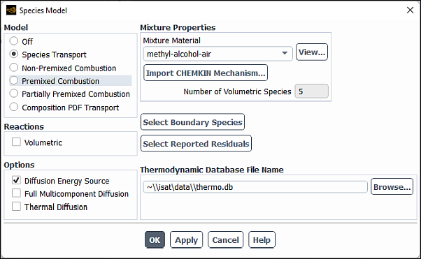
1. Select Species Transport in the Model list.
2. Select methyl-alcohol-air from the Mixture Material drop-down list.
  The Mixture Material list contains the set of chemical mixtures that exist in the Ansys Fluent database. When selecting an appropriate mixture for your case, you can review the constituent species and the reactions of the predefined mixture by clicking View... next to the Mixture Material drop-down list. The chemical species and their physical and thermodynamic properties are defined by the selection of the mixture material. After enabling the Species Transport model, you can alter the mixture material selection or modify the mixture material properties using the Create/Edit Materials dialog box. You will modify your local copy of the mixture material later in this tutorial.
3. Click OK to close the Species Model dialog box.

21.4.5. Materials

Define materials using the Materials task page.

Setup → Materials

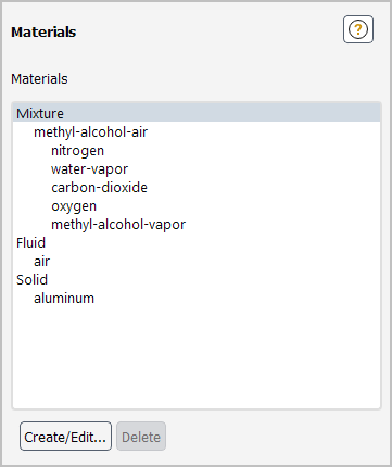
Edit the methyl-alcohol-air mixture material by removing water vapor and carbon dioxide from the mixture species list.
Setup → Materials → Mixture → Create/Edit...
1. In the Create/Edit Materials dialog box for the methyl-alcohol-air mixture material, click the Edit... button next to the Mixture Species drop-down list (Properties group box) to open the Species dialog box.
  1. In the Selected Species selection list, select carbon dioxide (co2).
  2. Click Remove to remove carbon dioxide from the Selected Species list.
  3. In a similar manner, remove water vapor (h2o) from the Selected Species list.
  4. Click OK to close the Species dialog box.
  5. Click OK in the Warning dialog box informing you that the species mixture has been modified and asking you to check the species boundary conditions.
2. Click Change/Create and close the Create/Edit Materials dialog box.
  Note: It is good practice to click the Change/Create button whenever changes are made to material properties even though it is not necessary in this case.

21.4.6. Boundary Conditions

Specify boundary conditions using the Boundary Conditions task page.

Setup → Boundary Conditions

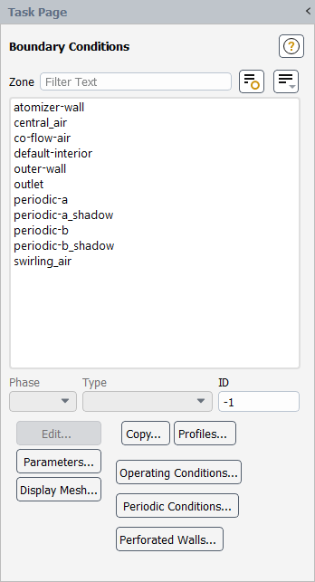
Set the boundary conditions for the inner air stream (central_air).
Setup → Boundary Conditions → central_air → Edit...
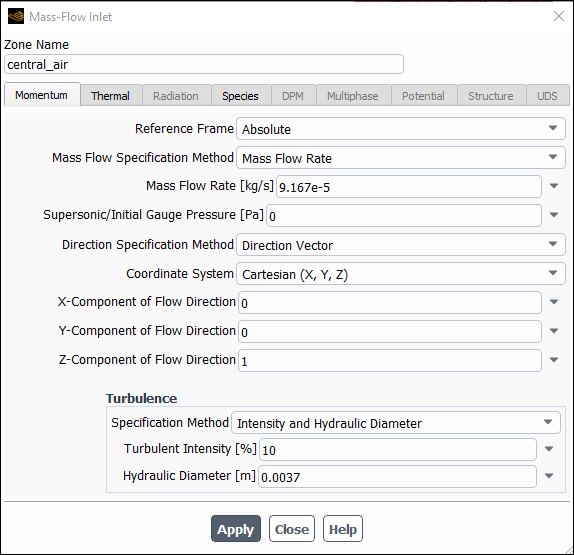
1. Enter 9.167e-5 kg/s for Mass Flow Rate.
2. Select Direction Vector for the Direction Specification Method.
3. Enter 0 for X-Component of Flow Direction.
4. Retain the default value of 0 for Y-Component of Flow Direction.
5. Enter 1 for Z-Component of Flow Direction.
6. Select Intensity and Hydraulic Diameter from the Specification Method drop-down list.
7. Enter 10 for Turbulent Intensity.
8. Enter 0.0037 m for Hydraulic Diameter.
9. Click the Thermal tab and enter 293 K for Total Temperature.
10. Click the Species tab and enter 0.23 for o2 in the Species Mass Fractions group box.
11. Click Apply and close the Mass-Flow Inlet dialog box.
Set the boundary conditions for the air stream surrounding the atomizer (co-flow-air).
Setup → Boundary Conditions → co-flow-air → Edit...
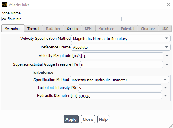
1. Enter 1 m/s for Velocity Magnitude.
2. Select Intensity and Hydraulic Diameter from the Specification Method drop-down list.
3. Retain the default value of 5 for Turbulent Intensity.
4. Enter 0.0726 m for Hydraulic Diameter.
5. Click the Thermal tab and enter 293 K for Temperature.
6. Click the Species tab and enter 0.23 for o2 in the Species Mass Fractions group box.
7. Click Apply and close the Velocity Inlet dialog box.
Set the boundary conditions for the exit boundary (outlet).
Setup → Boundary Conditions → outlet → Edit...
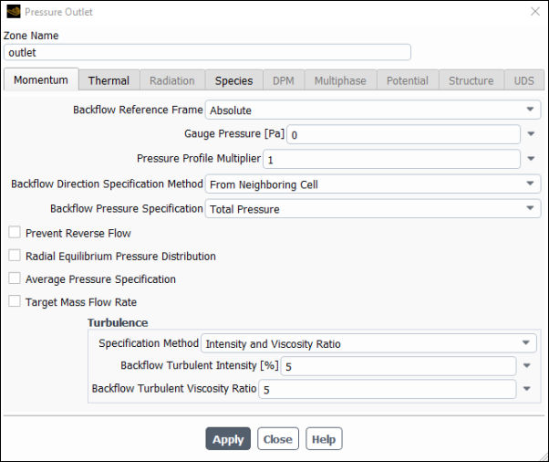
1. Select From Neighboring Cell from the Backflow Direction Specification Method drop-down list.
2. Retain Intensity and Viscosity Ratio from the Specification Method drop-down list.
3. Retain the default value of 5 for Backflow Turbulent Intensity (%).
4. Enter 5 for Backflow Turbulent Viscosity Ratio.
5. Click the Thermal tab and enter 293 K for Backflow Total Temperature.
6. Click the Species tab and enter 0.23 for o2 in the Species Mass Fractions group box.
7. Click Apply and close the Pressure Outlet dialog box.
Set the boundary conditions for the swirling annular stream (swirling_air).
Setup → Boundary Conditions → swirling_air → Edit...
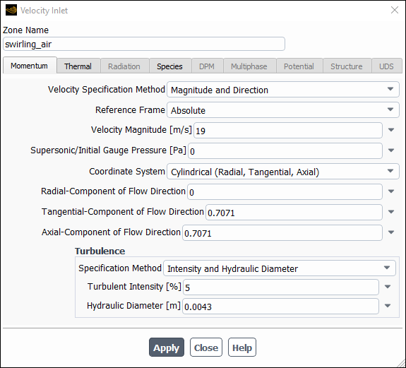
1. Select Magnitude and Direction from the Velocity Specification Method drop-down list.
2. Enter 19 m/s for Velocity Magnitude.
3. Select Cylindrical (Radial, Tangential, Axial) from the Coordinate System drop-down list.
4. Enter 0 for Radial-Component of Flow Direction.
5. Enter 0.7071 for Tangential-Component of Flow Direction.
6. Enter 0.7071 for Axial-Component of Flow Direction.
7. Select Intensity and Hydraulic Diameter from the Specification Method drop-down list.
8. Retain the default value of 5 for Turbulent Intensity.
9. Enter 0.0043 m for Hydraulic Diameter.
10. Click the Thermal tab and enter 293 K for Temperature.
11. Click the Species tab and enter 0.23 for o2 in the Species Mass Fractions group box.
12. Click Apply and close the Velocity Inlet dialog box.
Set the boundary conditions for the outer wall of the atomizer (outer-wall).
Setup → Boundary Conditions → outer-wall → Edit...
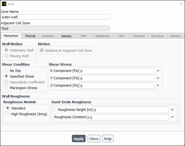
1. Select Specified Shear in the Shear Condition list.
2. Retain the default values for the remaining parameters.
3. Click Apply and close the Wall dialog box.

21.4.7. Initial Solution Without Droplets

The airflow will first be solved and analyzed without droplets.

Set the solution method.
Solution → Solution → Methods...

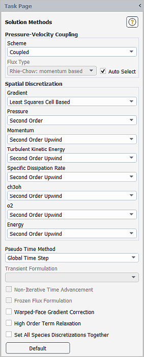
Retain the default selections.
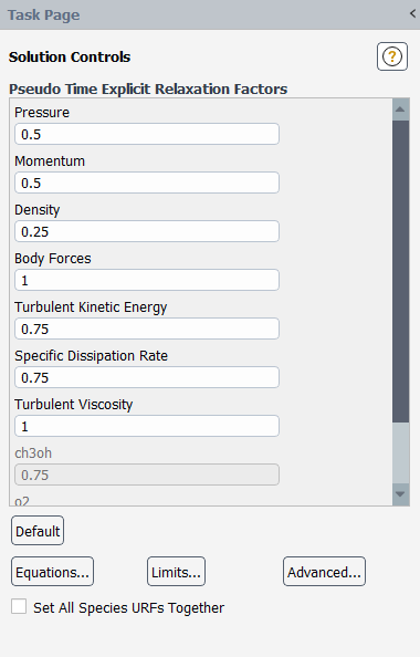
Retain the default under-relaxation factors.
Solution → Controls → Controls...
Enable residual plotting during the calculation.
Solution → Reports → Residuals...
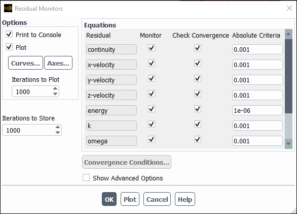
1. Ensure that Plot is enabled in the Options group box.
2. Click OK to close the Residual Monitors dialog box.
Initialize the flow field.
Solution → Initialization
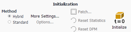
1. Retain the Method at the default of Hybrid.
2. Click Initialize to initialize the variables.
Note: For flows in complex topologies, hybrid initialization will provide better initial velocity and pressure fields than standard initialization. This will help to improve the convergence behavior of the solver.
Save the case file (spray1.cas.h5).
File → Write → Case...
Start the calculation by requesting 150 iterations.
Solution → Run Calculation
1. In the Fluid Time Scale group box, retain Automatic for Time Step Method and 1s for Time Scale Factor.
2. Enter 150 for Number of Iterations.
3. Click Calculate.
Figure 21.3: Scaled Residuals
Save the case and data files (spray1.cas.h5 and spray1.dat.h5).
File → Write → Case & Data...
Note: Ansys Fluent will ask you to confirm that the previous case file is to be overwritten.
Create a clip plane to examine the flow field at the midpoint of the atomizer section.
Results → Surface → Create → Iso-Surface...
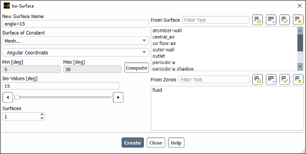
1. Enter angle=15 for New Surface Name.
2. Select Mesh... and Angular Coordinate from the Surface of Constant drop-down lists.
3. Click Compute to obtain the minimum and maximum values of the angular coordinate.
4. Enter 15 for Iso-Values.
5. Click Create to create the isosurface.
6. Close the Iso-Surface dialog box.
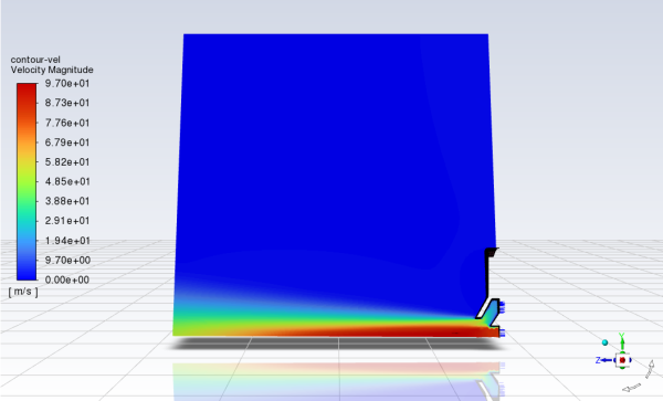
Review the current state of the solution by examining contours of velocity magnitude (Figure 21.4: Velocity Magnitude at Mid-Point of Atomizer Section).
Results → Graphics → Contours → New...
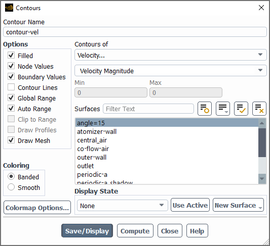
1. Enter contour-vel for Contour Name.
2. Select Banded in the Coloring group box.
3. Select Velocity... and Velocity Magnitude from the Contours of drop-down lists.
4. Enable Draw Mesh.
  The Mesh Display dialog box will open.
  1. Retain the current mesh display settings.
  2. Close the Mesh Display dialog box.
5. Select angle=15 from the Surfaces selection list.
6. Click Save/Display and close the Contours dialog box.
7. Use the mouse to obtain the view shown in Figure 21.4: Velocity Magnitude at Mid-Point of Atomizer Section.
Figure 21.4: Velocity Magnitude at Mid-Point of Atomizer Section
Display pathlines of the air in the swirling annular stream (Figure 21.5: Pathlines of Air in the Swirling Annular Stream).
Results → Graphics → Pathlines → New...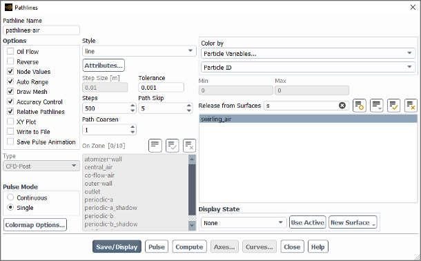
1. Enter pathlines-air for Pathline Name.
2. Increase the Path Skip value to 5.
3. In the Release from Surfaces filter, type s to display the surface names that begin with s and select swirling_air from the selection list.
4. Enable Draw Mesh in the Options group box.
  The Mesh Display dialog box will open.
  1. Retain the current mesh display settings.
  2. Close the Mesh Display dialog box.
5. Click Save/Display and close the Pathlines dialog box.
6. Use the mouse to obtain the view shown in Figure 21.5: Pathlines of Air in the Swirling Annular Stream.
  Figure 21.5: Pathlines of Air in the Swirling Annular Stream

21.4.8. Creating a Spray Injection

Define the discrete phase modeling parameters.
Physics → Models → Discrete Phase...
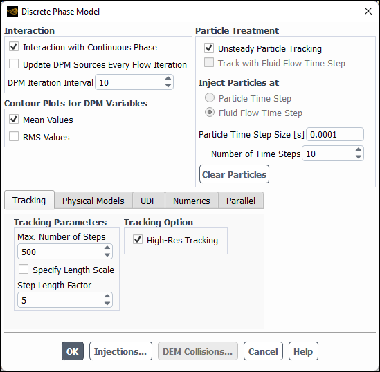
1. Select Interaction with Continuous Phase in the Interaction group box.
  This will include the effects of the discrete phase trajectories on the continuous phase.
2. Retain the value of 10 for DPM Iteration Interval.
3. Select Mean Values in the Contour Plots for DPM Variables group box.
  This will make the cell-averaged variables available for postprocessing activities.
4. In the Particle Treatment group box, select the Unsteady Particle Tracking option.
5. Enter 0.0001 for Particle Time Step Size.
6. Enter 10 for Number of Time Steps.
7. Under the Physical Models tab, enable Temperature Dependent Latent Heat and Breakup in the Options group box.
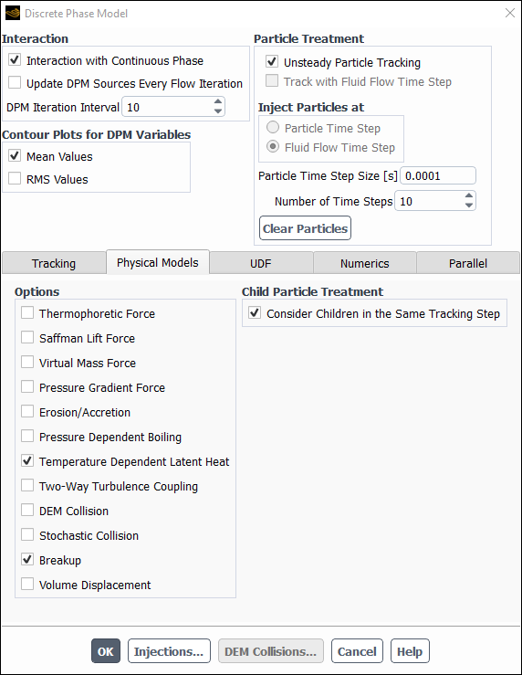
8. Under the Numerics tab, select Linearize Source Terms (Source Terms group).
  Enabling this option will allow you to run the simulation with more aggressive setting for the Discrete Phase Sources under-relaxation factor to speed up the solution convergence.
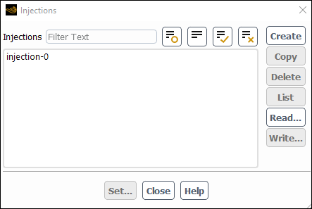
9. Click Injections... to open the Injections dialog box.
  In this step, you will define the characteristics of the atomizer.
  
  An Information dialog box appears indicating that the Max. Number of Steps has been changed from 50000 to 500. Click OK in the Information dialog box to continue.
10. Click the Create button to create the spray injection.
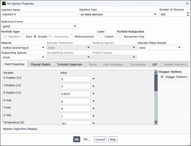
11. In the Set Injection Properties dialog box, select air-blast-atomizer from the Injection Type drop-down list.
12. Enter 600 for Number of Streams.
  This option controls the number of droplet parcels that are introduced into the domain at every time step.
13. In the Particle Type group box, select Droplet.
14. Select methyl-alcohol-liquid from the Material drop-down list.
15. In the Point Properties tab, specify point properties for particle injections.
  1. Retain the default values of 0 and 0 for X-Position and Y-Position.
  2. Enter 0.0015 for Z-Position.
  3. Retain the default values of 0, 0, and 1 for X-Axis, Y-Axis, and Z-Axis, respectively.
  4. Enter 263 K for Temperature.
    Scroll down the list to see the remaining point properties.
  5. Enter 8.5e-5 kg/s for Flow Rate.
    This is the methanol flow rate for a 30-degree section of the atomizer. The actual atomizer flow rate is 12 times this value.
  6. Retain the default Start Time of 0 s and enter 100 s for the Stop Time.
    For this problem, the injection should begin at and not stop until long after the time period of interest. A large value for the stop time (for example, 100 s) will ensure that the injection will essentially never stop.
  7. Enter 0.0035 m for the Injector Inner Diameter and 0.0045 m for the Injector Outer Diameter.
  8. Enter 45 degrees for Spray Half Angle.
    The spray angle is the angle between the liquid sheet trajectory and the injector centerline.
  9. Enter 82.6 m/s for the Relative Velocity.
    The relative velocity is the expected relative velocity between the atomizing air and the liquid sheet.
  10. Retain the default Azimuthal Start Angle of 0 degrees and enter 30 degrees for the Azimuthal Stop Angle.
    This will restrict the injection to the 30-degree section of the atomizer that is being modeled.
16. In the Physical Models tab, specify the breakup model and drag parameters.
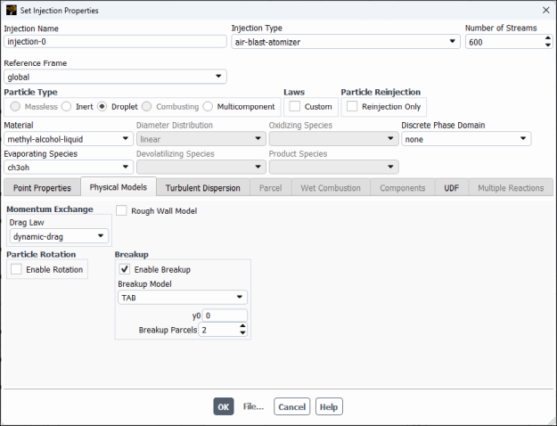
  1. In the Drag Parameters group box, select dynamic-drag from the Drag Law drop-down list.
    The dynamic-drag law is available only when the Breakup model is used.
  2. In the Breakup group, ensure that Enable Breakup is selected and TAB is selected from the Breakup Model drop-down list.
  3. Retain the default values of 0 for y0 and 2 for Breakup Parcels.
17. In the Turbulent Dispersion tab, define the turbulent dispersion.
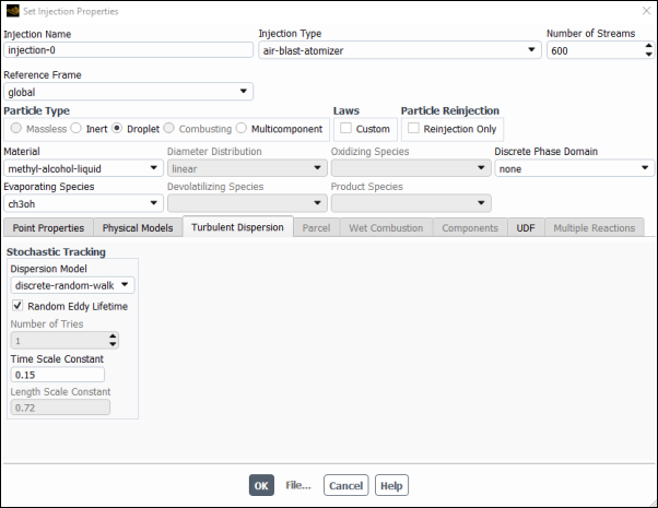
  1. Select Discrete Random Walk Model and enable Random Eddy Lifetime in the Stochastic Tracking group box.
    These models will account for the turbulent dispersion of the droplets.
  2. Click OK to close the Set Injection Properties dialog box.
    Note: If you want to modify the existing injection, then in the Injections dialog box, select its name in the Injections list and click Set..., or simply double-click the injection of interest.
18. Close the Injections dialog box.
  Note: In the case that the spray injection would be striking a wall, you must specify the wall boundary conditions for the droplets. Though this tutorial does have wall zones, they are a part of the atomizer apparatus. You need not change the wall boundary conditions any further because these walls are not in the path of the spray droplets.
19. Click OK to close the Discrete Phase Model dialog box.
Specify the droplet material properties.
Setup → Materials → methyl-alcohol-liquid → Create/Edit...
When secondary atomization models (such as Breakup) are used, several droplet properties need to be specified.
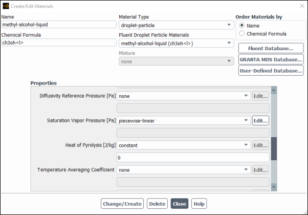
1. Ensure droplet-particle is selected in the Material Type drop-down list.
2. Enter 0.00095 kg/m-s for Viscosity in the Properties group box.
3. Ensure that piecewise-linear is selected from the Saturation Vapor Pressure drop-down list.
  Scroll down to find the Saturation Vapor Pressure drop-down list.
4. Click the Edit... button next to Saturation Vapor Pressure to open the Piecewise-Linear Profile dialog box.
5. Retain the default values and click OK to close the Piecewise-Linear Profile dialog box.
6. Select convection/diffusion-controlled from the Vaporization/Boiling Model drop-down list.
7. Click OK to close the Model Options dialog box.
8. Click Change/Create to accept the change in properties for the methanol droplet material and close the Create/Edit Materials dialog box.

21.4.9. Solution

Increase the under-relaxation factor for Discrete Phase Sources.
Solution → Controls → Controls...
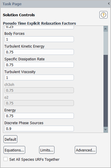
In the Pseudo Time Explicit Relaxation Factors group box, change the under-relaxation factor for Discrete Phase Sources to 0.9.
Remove the convergence criteria.
Solution → Reports → Residuals...
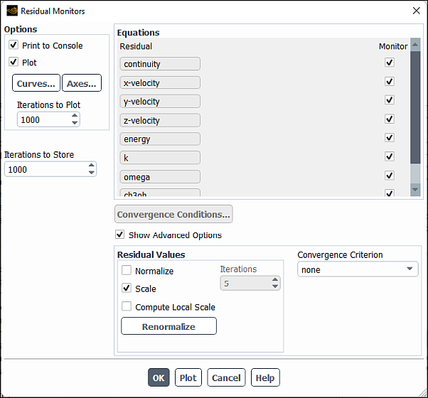
1. Enable Show Advanced Options and select none from the Convergence Criterion drop-down list.
2. Click OK to close the Residual Monitors dialog box.
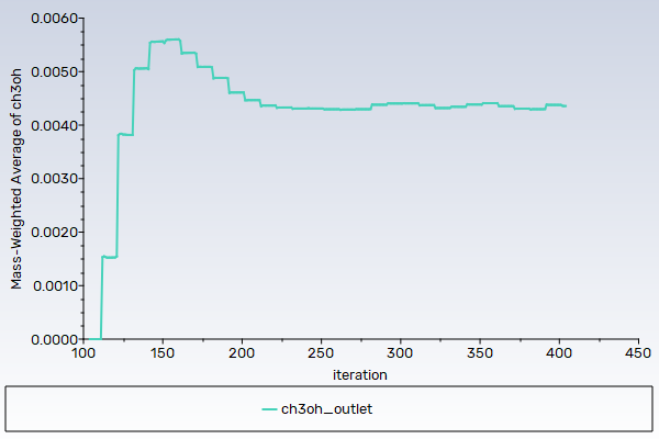
Enable the plotting of mass fraction of ch3oh.
Solution → Reports → Definitions → New → Surface Report → Mass-Weighted Average...
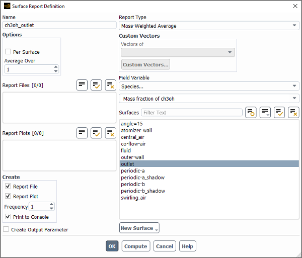
1. Enter ch3oh_outlet for Name of the surface report definition.
2. In the Create group box, enable Report Plot and Print to Console.
3. Select Species... and Mass fraction of ch3oh from the Field Variable drop-down lists.
4. Select outlet from the Surfaces selection list.
5. Click OK to save the surface report definition settings and close the Surface Report Definition dialog box.
  Fluent automatically generates the ch3oh_outlet-rplot report plot under the Solution/Monitors/Report Plots tree branch.
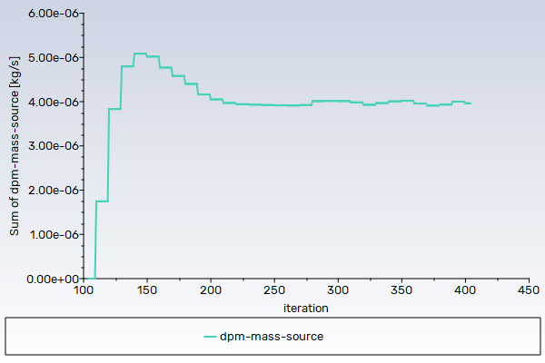
Enable the plotting of the sum of the DPM Mass Source.
Solution → Reports → Definitions → New → Volume Report → Sum...
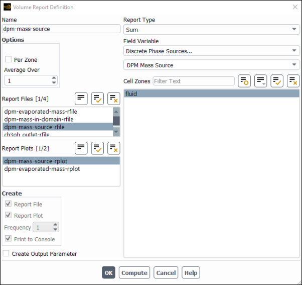
1. Enter dpm-mass-source for Name.
2. In the Create group box, enable Report Plot and Print to Console.
3. Select Discrete Phase Sources... and DPM Mass Source from the Field Variable drop-down lists.
4. Select fluid from the Cell Zones selection list.
5. Click OK to save the volume report definition settings and close the Volume Report Definition dialog box.
  Fluent automatically generates the dpm-mass-source-rplot report plot under Solution/Monitors/Report Plots tree branch.
6. Modify the attributes of the dpm-mass-source-rplot report plot axes.
  Solution → Monitors → Report Plots → dpm-mass-source-rplot Edit...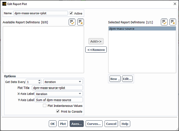
  1. Click the Axes... button to open the Axes dialog box.
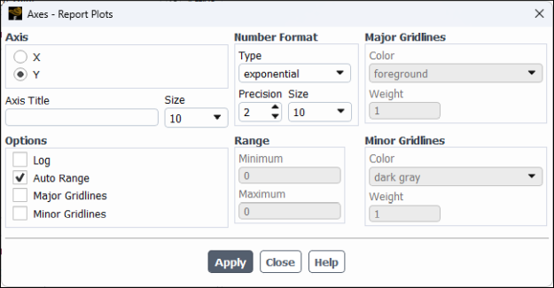
  2. Select Y in the Axis list.
  3. Select exponential from the Type drop-down list.
  4. Set Precision to 2.
  5. Click Apply and close the Axes dialog box.
  6. Click OK to close the Edit Report Plot dialog box.
Create a DPM report definition for tracking the total mass present in the domain.
Solution → Reports → Definitions → New → DPM Report → Mass in Domain...
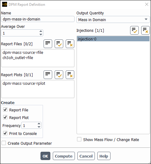
1. Enter dpm-mass-in-domain for Name.
2. In the Create group box, enable Report Plot and Print to Console.
3. Select injection-0 from the Injections selection list.
4. Disable Show Mass Flow / Change Rate.
5. Click OK to save the volume report definition settings and close the DPM Report Definition dialog box.
  Fluent automatically generates the dpm-mass-in-domain-rplot report plot under Solution/Monitors/Report Plots tree branch.
6. Modify the attributes of the dpm-mass-in-domain-rplot report plot axes (in a manner similar to that for the dpm-mass-source-rplot plot).
  Solution → Monitors → Report Plots → dpm-mass-in-domain-rplot Edit...
  1. In the Plot Window group box, click the Axes... button to open the Axes dialog box.
  2. Select Y in the Axis list.
  3. Select exponential from the Type drop-down list.
  4. Set Precision to 2.
  5. Click Apply and close the Axes dialog box.
  6. Click OK to close the Edit Report Plot dialog box.
Create a DPM report definition for tracking the mass of the evaporated particles.
Solution → Reports → Definitions → New → DPM Report → Evaporated Mass...
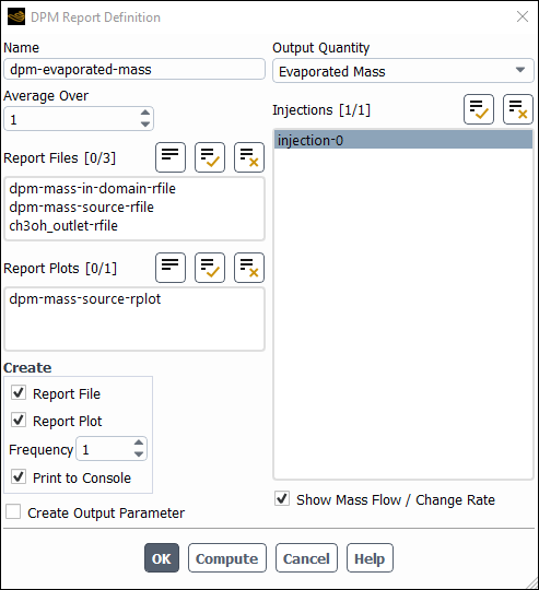
1. Enter dpm-evaporated-mass for Name.
2. In the Create group box, enable Report Plot and Print to Console.
3. Select injection-0 from the Injections selection list.
4. Ensure that the Show Mass Flow / Change Rate option is selected.
5. Click OK to save the volume report definition settings and close the DPM Report Definition dialog box.
  Fluent automatically generates the dpm-evaporated-mass-rplot report plot under Solution/Monitors/Report Plots tree branch.
6. Modify the attributes of the dpm-evaporated-mass-rplot report plot axes in a manner similar to that for the dpm-mass-source-rplot plot.
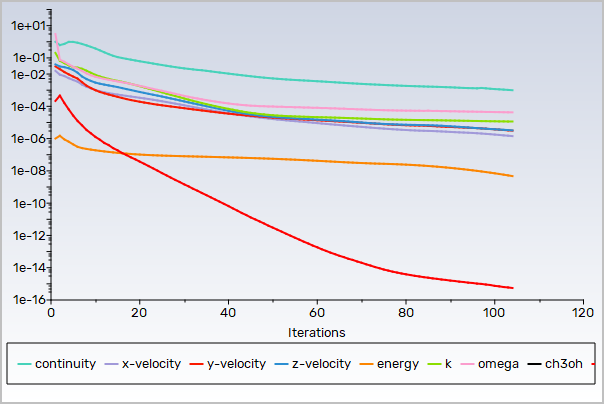
Request 300 more iterations (Figure 21.6: Convergence History of Mass Fraction of ch3oh on Fluid, Figure 21.7: Convergence History of DPM Mass Source on Fluid, Figure 21.8: Convergence History of Total Mass in Domain, and Figure 21.9: Convergence History of Evaporated Particle Mass).
Solution → Run Calculation
It can be concluded that the solution is converged because the number of particle tracks are constant and the flow variable plots are flat.
Figure 21.6: Convergence History of Mass Fraction of ch3oh on Fluid

Figure 21.7: Convergence History of DPM Mass Source on Fluid

Figure 21.8: Convergence History of Total Mass in Domain

Figure 21.9: Convergence History of Evaporated Particle Mass
Save the case and data files (spray2.cas.h5 and spray2.dat.h5).
File → Write → Case & Data...

21.4.10. Postprocessing

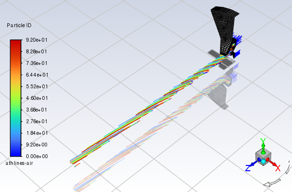
Display the trajectories of the droplets in the spray injection (Figure 21.10: Particle Tracks for the Spray Injection).
This will allow you to review the location of the droplets.
Results → Graphics → Particle Tracks → New...
1. Enter particle-tracks-droplets for Particle Tracks Name.
2. Enable Draw Mesh in the Options group box.
  The Mesh Display dialog box will open.
  1. Retain the current display settings.
  2. Close the Mesh Display dialog box.
3. Retain the default selection of point from the Track Style drop-down list.
4. Select Particle Variables... and Particle Diameter from the Color by drop-down lists.
  This will display the location of the droplets colored by their diameters.
5. Select injection-0 from the Release from Injections selection list.
6. Click Save/Display.
  As an optional exercise, you can increase the particle size by clicking the Attributes... button in the Particle Tracks dialog box and adjusting the Marker Size value in the Track Style Attributes dialog box.
7. Close the Particle Tracks dialog box.
8. Use the mouse to obtain the view shown in Figure 21.10: Particle Tracks for the Spray Injection.
Figure 21.10: Particle Tracks for the Spray Injection

The air-blast atomizer model assumes that a cylindrical liquid sheet exits the atomizer, which then disintegrates into ligaments and droplets. Appropriately, the model determines that the droplets should be input into the domain in a ring. The radius of this disk is determined from the inner and outer radii of the injector.
Note: In the real device, the inner diameter and outer diameter of the liquid injection are 3.5 mm and 4.5 mm, respectively. Hence a liquid sheet is formed that is about 0.5 mm in thickness. The shear forces of the two air streams quickly disperse the liquid into droplets between, roughly, 4 µm and 50 µm in diameter. This is predicted by the air-blast-atomizer model, which uses the parameters specified in the "Set Injection Properties" dialog box.
Also note that the droplets are placed a slight distance away from the injector. Once the droplets are injected into the domain, their behavior will be determined by secondary models. For instance, they may collide/coalesce with other droplets depending on the secondary models employed. However, once a droplet has been introduced into the domain, the air-blast atomizer model no longer affects the droplet.
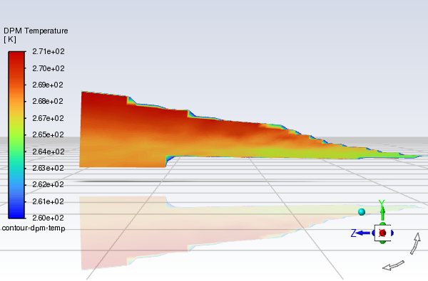
Display the mean particle temperature field (Figure 21.11: Contours of DPM Temperature).
Results → Graphics → Contours → New...
1. Enter contour-dpm-temp for Contour Name.
2. Ensure that Filled is enabled in the Options group box.
3. Select Banded in the Coloring group box.
4. Select Discrete Phase Variables... and DPM Temperature from the Contours of drop-down lists.
5. Disable Auto Range.
  The Clip to Range option will automatically be enabled.
6. Click Compute to update the Min and Max fields.
7. Enter 260 for Min.
8. Select angle=15 from the Surfaces selection list.
9. Click Save/Display and close the Contours dialog box.
10. Use the mouse to obtain the view shown in Figure 21.11: Contours of DPM Temperature.
Figure 21.11: Contours of DPM Temperature
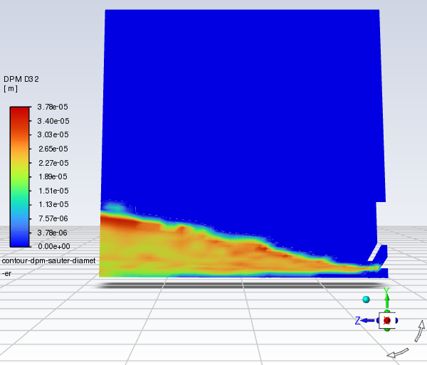
Display the mean Sauter diameter (Figure 21.12: Contours of DPM Sauter Diameter).
Results → Graphics → Contours → New...
1. Enter contour-dpm-sauter-diameter for Contour Name.
2. Ensure that Filled is enabled in the Options group box.
3. Select Banded in the Coloring group box.
4. Select Discrete Phase Variables... and DPM D32 from the Contours of drop-down lists.
5. Select angle=15 from the Surfaces selection list.
6. Click Save/Display and close the Contours dialog box.
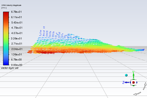
Figure 21.12: Contours of DPM Sauter Diameter
Display vectors of DPM mean velocity colored by DPM velocity magnitude (Figure 21.13: Vectors of DPM Mean Velocity Colored by DPM Velocity Magnitude).
Results → Graphics → Vectors → New...
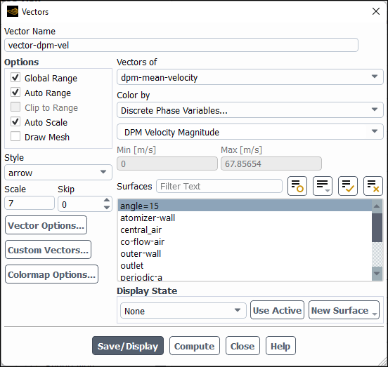
1. Enter vector-dpm-vel for Vector Name.
2. Select dpm-mean-velocity from the Vectors of drop-down lists.
3. Select Discrete Phase Variables... and DPM Velocity Magnitude from the Color by drop-down lists.
4. Select arrow from the Style drop-down list.
5. Enter 7 for Scale.
6. Select angle=15 from the Surfaces selection list.
7. Click Save/Display and close the Vectors dialog box.
Figure 21.13: Vectors of DPM Mean Velocity Colored by DPM Velocity Magnitude
Create an isosurface of the methanol mass fraction.
Results → Surface → Create → Iso-Surface...
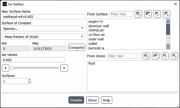
1. Enter methanol-mf=0.002 for the New Surface Name.
2. Select Species... and Mass fraction of ch3oh from the Surface of Constant drop-down lists.
3. Click Compute to update the minimum and maximum values.
4. Enter 0.002 for Iso-Values.
5. Click Create and then close the Iso-Surface dialog box.
Display the isosurface you just created (methanol-mf=0.002).
Results → Graphics → Mesh → New...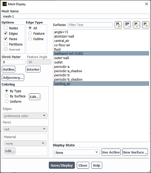
1. Deselect atomizer-wall and central_air in the Surfaces selection list.
2. Select methanol-mf=0.002 and swirling_air in the Surfaces selection list.
3. Click Save/Display in the Mesh Display dialog box.
  The graphics display will be updated to show the isosurface.
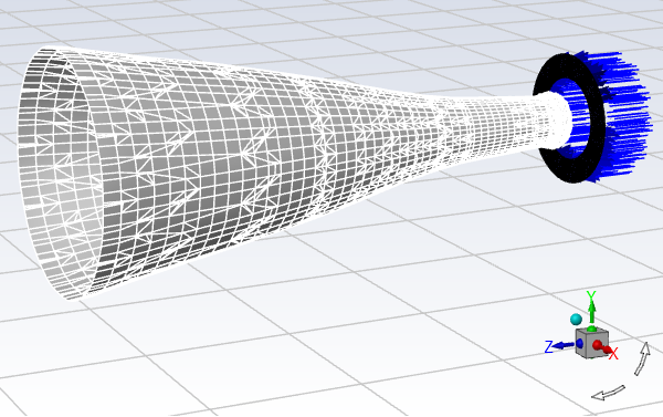
Modify the view to include the entire atomizer.
View → Display → Periodic Instancing...
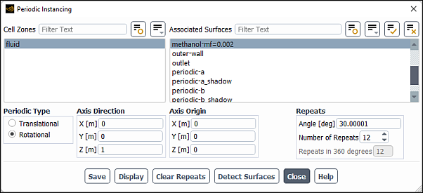
1. Select fluid from the Cell Zones list.
2. Select swirling_air and methanol-mf=0.002 from the Associated Surfaces selection list.
3. Retain the selection of Rotational in the Periodic Type list.
4. Set 12 for the Number of Repeats.
5. Click Save and close the Periodic Instancing dialog box.
6. Click Display and close the Mesh Display dialog box.
7. Use the mouse to obtain the view shown in Figure 21.14: Full Atomizer Display with Surface of Constant Methanol Mass Fraction.
  Figure 21.14: Full Atomizer Display with Surface of Constant Methanol Mass Fraction
8. This view can be improved to resemble Figure 21.15: Atomizer Display with Surface of Constant Methanol Mass Fraction Enhanced by changing some of the following variables:
  1. Open the mesh-1 object you saved earlier.
    Results → Graphics → Mesh → mesh-1 Edit...
  2. In the Mesh Display dialog box, disable Edges.
  3. Click Save/Display.
  4. In the Periodic Instancing dialog box, change the Number of Repeats to 6.
    View → Display → Periodic Instancing...
  5. Make sure that swirling_air and methanol-mf=0.002 are selected in the Surfaces list.
  6. Click Display.
  7. In the View ribbon tab, enable the Headlight and Lighting display options and change lighting to Flat (Display group).
  Figure 21.15: Atomizer Display with Surface of Constant Methanol Mass Fraction Enhanced
Save the case and data files (spray3.cas.h5 and spray3.dat.h5).
File → Write → Case & Data...

21.5. Summary

In this tutorial, a spray injection was defined for an air-blast atomizer and the solution was calculated using the discrete phase model in Ansys Fluent. The location of methanol droplet particles after exiting the atomizer and an isosurface of the methanol mass fraction were examined.