Chapter 22: Using the VOF Model

This tutorial is divided into the following sections:

22.1. Introduction

This tutorial examines the flow of ink as it is ejected from the nozzle of a printhead in an inkjet printer. Using Ansys Fluent’s volume of fluid (VOF) multiphase modeling capability, you will be able to predict the shape and motion of the resulting droplets in an air chamber.

This tutorial demonstrates how to do the following:

Set up and solve a transient problem using the pressure-based solver and VOF model.
Copy material from the property database.
Define time-dependent boundary conditions with an expression.
Patch initial conditions in a subset of the domain.
Automatically save data files at defined points during the solution.
Examine the flow and interface of the two fluids using volume fraction contours.

22.2. Prerequisites

This tutorial is written with the assumption that you have completed the introductory tutorials found in this manual and that you are familiar with the Ansys Fluent outline view and ribbon structure. Some steps in the setup and solution procedure will not be shown explicitly.

22.3. Problem Description

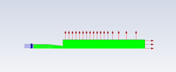
The problem considers the transient tracking of a liquid-gas interface in the geometry shown in Figure 22.1: Schematic of the Problem. The axial symmetry of the problem enables a 2D geometry to be used. The computation mesh consists of 24,600 cells. The domain consists of two regions: an ink chamber and an air chamber. The dimensions are summarized in Table 22.1: Ink Chamber Dimensions.

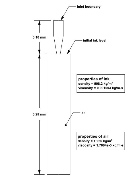
Figure 22.1: Schematic of the Problem

Table 22.1: Ink Chamber Dimensions

Ink Chamber, Cylindrical Region: Radius (mm)	0.015
Ink Chamber, Cylindrical Region: Length (mm)	0.050
Ink Chamber, Tapered Region: Final Radius (mm)	0.009
Ink Chamber, Tapered Region: Length (mm)	0.050
Air Chamber: Radius (mm)	0.030
Air Chamber: Length (mm)	0.280

The following is the chronology of events modeled in this simulation:

At time zero, the nozzle is filled with ink, while the rest of the domain is filled with air. Both fluids are assumed to be at rest. To initiate the ejection, the ink velocity at the inlet boundary (which is modeled in this simulation by a user-defined function) suddenly increases from 0 to 3.58 m/s and then decreases according to a cosine law.
After 10 microseconds, the velocity returns to zero.

The calculation is run for 30 microseconds overall, that is, three times longer than the duration of the initial impulse.

Because the dimensions are small, the double-precision version of Ansys Fluent will be used. Air will be designated as the primary phase, and ink (which will be modeled with the properties of liquid water) will be designated as the secondary phase. Patching will be required to fill the ink chamber with the secondary phase. Gravity will not be included in the simulation. To capture the capillary effect of the ejected ink, the surface tension and prescription of the wetting angle will be specified. The surface inside the nozzle will be modeled as neutrally wettable, while the surface surrounding the nozzle orifice will be non-wettable.

22.4. Setup and Solution

The following sections describe the setup and solution steps for this tutorial:

22.4.1. Preparation

To prepare for running this tutorial:

Download the vof.zip file here .
Unzip vof.zip to your working directory.
The mesh file inkjet.msh can be found in the folder.
Use the Fluent Launcher to start Ansys Fluent.
Select Solution in the top-left selection list to start Fluent in Solution Mode.
Select 2D under Dimension.
Enable Double Precision under Options.
Note: The double precision solver is recommended for modeling multiphase flows simulation.
Set Solver Processes to 1 under Parallel (Local Machine).

22.4.2. Reading and Manipulating the Mesh

Read the mesh file inkjet.msh.
File → Read → Mesh...
Examine the mesh (Figure 22.2: Default Display of the Nozzle Mesh).
Figure 22.2: Default Display of the Nozzle Mesh

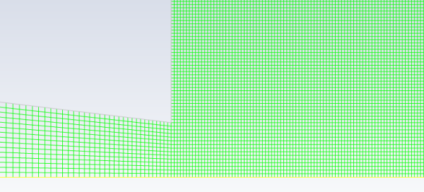
Tip: Zoom in by dragging the middle mouse button with the Shift key pressed, so that you can see that the interior of the model is composed of a fine mesh of quadrilateral cells (see Figure 22.3: The Quadrilateral Mesh).
Figure 22.3: The Quadrilateral Mesh
Set the graphics display options.
View → Display → Options...
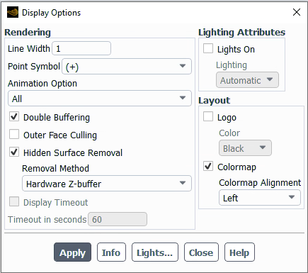
1. Ensure that All is selected from the Animation Option drop-down list.
  Selecting All will allow you to see the movement of the entire mesh as you manipulate the Camera view in the next step.
Click Apply and close the Display Options dialog box.
Manipulate the mesh display to show the full chamber upright.
View → Display → Views...
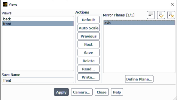
1. Select front from the Views selection list.
2. Select axis from the Mirror Planes selection list.
3. Click Apply.
  The mesh display is updated to show both sides of the chamber.
4. Click the Camera... button to open the Camera Parameters dialog box.
  
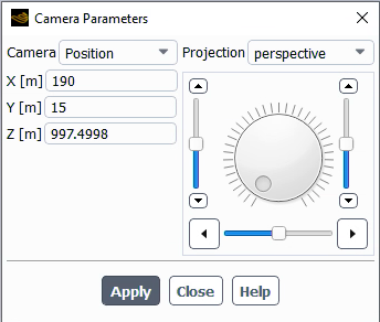
  Note: You may notice that the scale of the dimensions in the Camera Parameters dialog box appear very large given the problem dimensions. This is because you have not yet scaled the mesh to the correct units. You will do this in a later step.
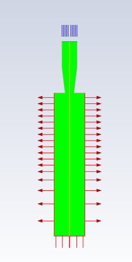
  1. Drag the indicator of the dial with the left mouse button in the clockwise direction until the upright view is displayed (Figure 22.4: Mesh Display of the Nozzle Mirrored and Upright).
    Figure 22.4: Mesh Display of the Nozzle Mirrored and Upright
  2. Click Apply and close the Camera Parameters dialog box.
5. Close the Views dialog box.

22.4.3. General Settings

Check the mesh.
Domain → Mesh → Check → Perform Mesh Check
Ansys Fluent will perform various checks on the mesh and report the progress in the console. Make sure that the reported minimum volume is a positive number.
Scale the mesh.
Domain → Mesh → Scale...
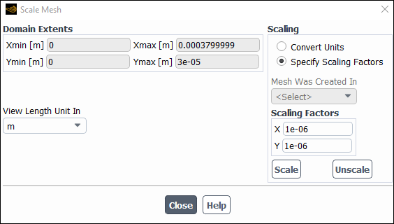
1. Select Specify Scaling Factors from the Scaling group box.
2. Enter 1e-6 for X and Y in the Scaling Factors group box.
3. Click Scale and close the Scale Mesh dialog box.
4. Right-click in the graphics window and select Refresh Display
5. Click the Fit to Window icon, , to center the graphic in the window.
Check the mesh.
Domain → Mesh → Check → Perform Mesh Check
Note: It is a good idea to check the mesh after you manipulate it (that is, scale, convert to polyhedra, merge, separate, fuse, add zones, or smooth and swap.) This will ensure that the quality of the mesh has not been compromised.
Define the units for the mesh.
Domain → Mesh → Units...
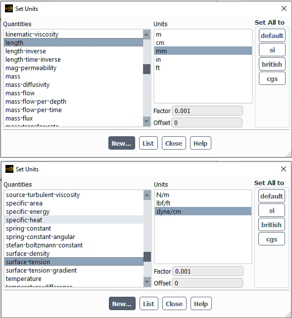
1. Select length from the Quantities list.
2. Select mm from the Units list.
3. Select surface-tension from the Quantities list.
4. Select dyne/cm from the Units list.
5. Close the Set Units dialog box.
Retain the default setting of Pressure-Based in the Solver group box of the General task page.
Setup → General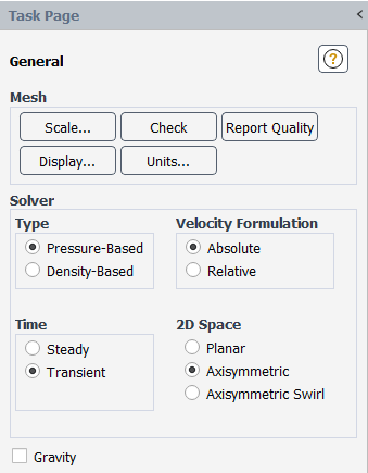
Select Transient from the Time list.
Select Axisymmetric from the 2D Space list.

22.4.4. Models

Enable the laminar viscous model.
Physics → Models → Viscous...
1. Select Laminar in the Model group box.
2. Click OK to close the Viscous Model dialog box.
Enable the Volume of Fluid multiphase model.
Physics → Models → Multiphase...
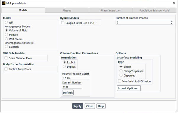
1. Select Volume of Fluid from the Model list.
  The Multiphase Model dialog box expands to show related inputs.
2. Retain the default settings and click Apply and close the Multiphase Model dialog box.
  Important: When setting up your case, if you have made changes in the current tab, you should click the Apply button to make them effective before moving to the next tab. Otherwise, the relevant models may not be available in the other tabs, and your settings may be lost.

22.4.5. Materials

The default properties of air and water defined in Ansys Fluent are suitable for this problem. In this step, you will make sure that both materials are available for selection in later steps.

Add water to the list of fluid materials by copying it from the Ansys Fluent materials database.
Physics → Materials → Create/Edit...
1. Click Fluent Database... in the Create/Edit Materials dialog box to open the Fluent Database Materials dialog box.
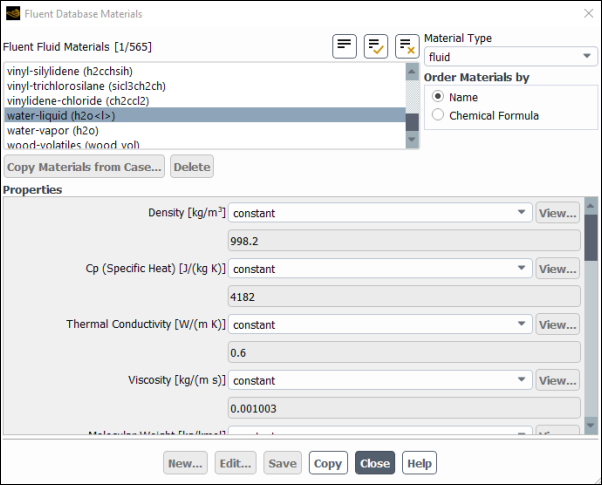
  1. Select water-liquid (h2o < l >) from the Fluent Fluid Materials selection list.
    Scroll down the Fluent Fluid Materials list to locate water-liquid (h2o < l >).
  2. Click Copy to copy the information for water to your list of fluid materials.
  3. Close the Fluent Database Materials dialog box.
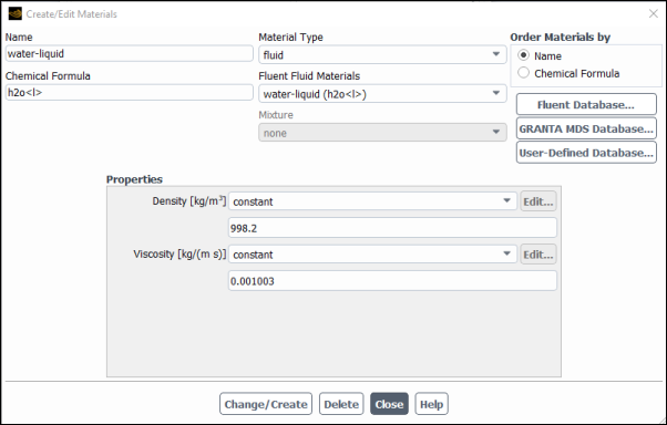
2. Click Change/Create and close the Create/Edit Materials dialog box.

22.4.6. Phases

In the following steps, you will define water as the secondary phase. When you define the initial solution, you will patch water in the nozzle region. In general, you can specify the primary and secondary phases whichever way you prefer. It is a good idea to consider how your choice will affect the ease of problem setup, especially with more complicated problems.

Physics → Models → Multiphase...

In the Multiphase Model dialog box, open the Phases tab.

Specify air (air) as the primary phase.
1. Select phase-1 – Primary Phase in the Phases selection list.
2. Enter air for Name.
3. Retain the default selection of air in the Phase Material drop-down list.
4. Click Apply
Specify water (water-liquid) as the secondary phase.
1. In the Phases selection list, select phase-2 – Secondary Phase.
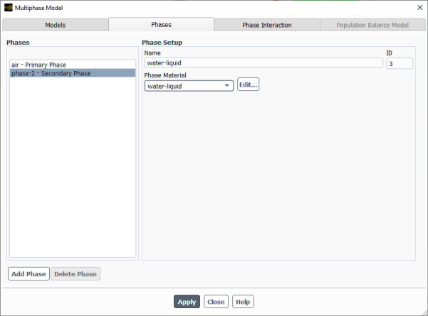
2. Enter water-liquid for Name.
3. Select water-liquid from the Phase Material drop-down list.
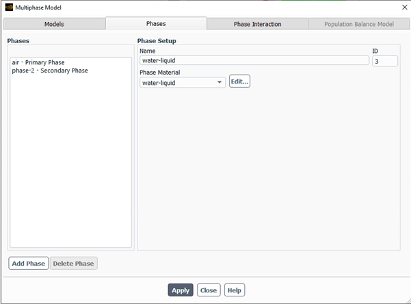
4. Click Apply.
Specify the interphase interaction.
In the Multiphase Model dialog box, open the Phase Interaction tab.
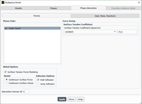
1. In the Force tab, select Surface Tension Force Modeling (Global Options group box).
  The surface tension inputs is displayed and the Continuum Surface Force model is set as the default.
2. Enable Wall Adhesion (Adhesion Options group box) so that contact angles can be prescribed.
3. For Surface Tension Coefficient (Force Setup group box), select constant from the drop-down list and enter 73.5 dyne/cm .
4. Click Apply.
Close the Multiphase Model dialog box.

22.4.7. Operating Conditions

Set the operating reference pressure location.
Setup → Boundary Conditions → Operating Conditions...

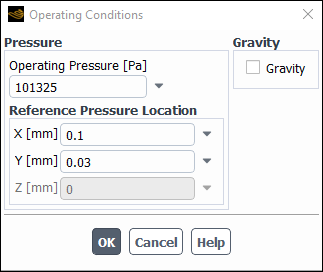
You will set the Reference Pressure Location to be a point where the fluid will always be 100 air.
1. Enter 0.10 mm for X.
2. Enter 0.03 mm for Y.
3. Click OK to close the Operating Conditions dialog box.

22.4.8. Boundary Conditions

Set the boundary conditions at the inlet (inlet) for the mixture by selecting mixture from the Phase drop-down list in the Boundary Conditions task page.
Setup → Boundary Conditions → Inlet → inlet Edit...
1. Select expression from the Velocity Magnitude drop-down list.
2. Enter the expression in the Expression Editor dialog box as shown and click OK and close the dialog box.
  IF(t<=10e-06[sec],3.58[m/s]*cos(PI*t/30e-6[s]),0[m/s])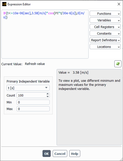
3. Click Apply and close the Velocity Inlet dialog box.
Set the boundary conditions at the inlet (inlet) for the secondary phase by selecting water-liquid from the Phase drop-down list in the Boundary Conditions task page.
Setup → Boundary Conditions → Inlet → inlet → water-liquid Edit...
1. Click the Multiphase tab and enter 1 for the Volume Fraction.
2. Click Apply and close the Velocity Inlet dialog box.
Set the boundary conditions at the outlet (outlet) for the secondary phase by selecting water-liquid from the Phase drop-down list in the Boundary Conditions task page.
Setup → Boundary Conditions → Outlet → outlet → water-liquid Edit...
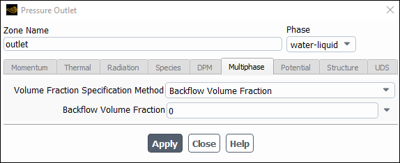
1. Click the Multiphase tab and retain the default setting of 0 for the Backflow Volume Fraction.
2. Click Apply and close the Pressure Outlet dialog box.
Set the conditions at the top wall of the air chamber (wall_no_wet) for the mixture by selecting mixture from the Phase drop-down list in the Boundary Conditions task page.
Setup → Boundary Conditions → Wall → wall_no_wet Edit...
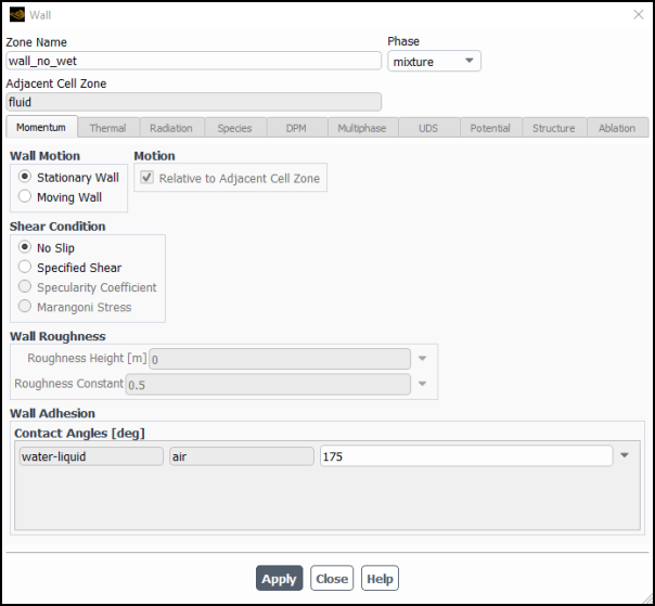
1. Enter 175 degrees for Contact Angles [deg].
2. Click Apply and close the Wall dialog box.
  Note: This angle affects the dynamics of droplet formation. You can repeat this simulation to find out how the result changes when the wall is hydrophilic (that is, using a small contact angle, say 10 degrees).
Set the conditions at the side wall of the ink chamber (wall_wet) for the mixture.
Setup → Boundary Conditions → Wall → wall_wet Edit...
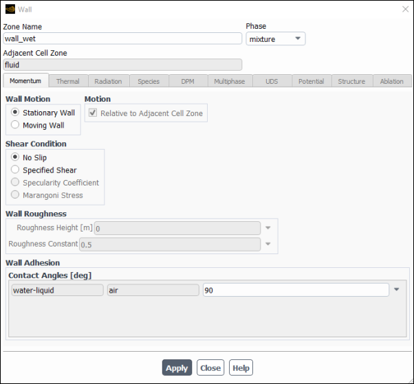
1. Retain the default setting of 90 degrees for Contact Angles [deg].
2. Click Apply and close the Wall dialog box.

22.4.9. Solution

Set the solution methods.
Solution → Solution → Methods...
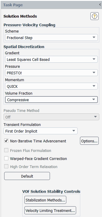
1. Enable Non-Iterative Time Advancement.
  The non-iterative time advancement (NITA) scheme is often advantageous compared to the iterative schemes as it is less CPU intensive. Although smaller time steps must be used with NITA compared to the iterative schemes, the total CPU expense is often smaller. If the NITA scheme leads to convergence difficulties, then the iterative schemes (for example, PISO, SIMPLE) should be used instead.
2. Select Fractional Step from the Scheme drop-down list in the Pressure-Velocity Coupling group box.
3. Retain the default selection of Least Squares Cell Based from the Gradient drop-down list in the Spatial Discretization group box.
4. Retain the default selection of PRESTO! from the Pressure drop-down list.
5. Select QUICK from the Momentum drop-down list.
6. Select Compressive from the Volume-Fraction drop-down list.
Enable the plotting of residuals during the calculation.
Solution → Reports → Residuals...
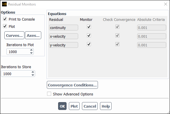
1. Ensure Plot is selected in the Options group box.
2. Click OK to close the Residual Monitors dialog box.
Initialize the solution after reviewing the default initial values.
Solution → Initialization → Options...
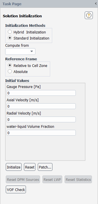
1. Retain the default settings for all the parameters and click Initialize (either in the ribbon or in the Solution Initialization task page.
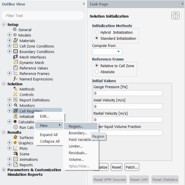
Define a register for the ink chamber region.
Solution → Cell Registers New → Region...
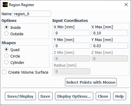
1. Enter a setting of 0 mm for X Min and Y Min in the Input Coordinates group box.
2. Enter 0.10 mm for X Max.
3. Enter 0.03 mm for Y Max.
4. Click Save and close the Region Register dialog box.
Patch the initial distribution of the secondary phase (water-liquid).
Solution → Initialization → Patch...
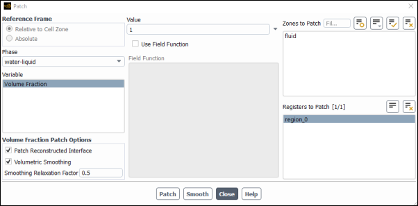
1. Select water-liquid from the Phase drop-down list.
2. Select Volume Fraction from the Variable list.
3. Enter 1 for Value.
4. Select region_0 from the Registers to Patch selection list.
5. Click Patch and close the Patch dialog box.
Request the saving of data files every 200 steps.
Solution → Activities → Autosave...
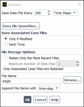
1. Enter 200 for Save Data File Every (Time Steps).
2. Ensure that time-step is selected from the Append File Name with drop-down list.
3. Enter inkjet for the File Name.
  Ansys Fluent will append the time step value to the file name prefix (inkjet). The standard .dat.h5 extension will also be appended. This will yield file names of the form inkjet-1-00200.dat.h5, where 200 is the time step number.
4. Click OK to close the Autosave dialog box.
Save the initial case file (inkjet.cas.h5).
File → Write → Case...
Run the calculation.
Solution → Run Calculation
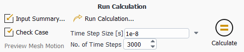
1. Enter 1e-8 seconds for the Time Step Size (s).
  Note: Small time steps are required to capture the oscillation of the droplet interface and the associated high velocities. Failure to use sufficiently small time steps may cause differences in the results between platforms.
2. Enter 3000 for the Number of Time Steps.
3. Click Calculate.
  The solution will run for 3000 iterations.

22.4.10. Postprocessing

Read the data file for the solution after 6 microseconds (inkjet-1-00600.dat.h5).
File → Read → Data...
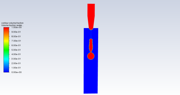
Create and display a filled contour of water volume fraction after 6 microseconds (Figure 22.5: Contours of Water Volume Fraction After 6 μs).
Results → Graphics → Contours → New...
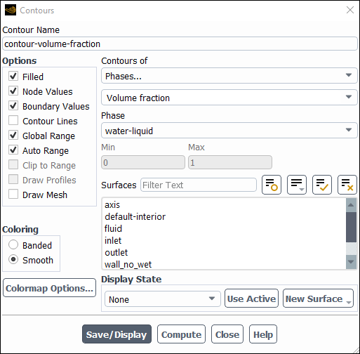
1. Change the Contour Name to contour-volume-fraction.
2. Enable Filled in the Options group box.
3. Select Phases... and Volume fraction from the Contours of drop-down lists.
4. Select water-liquid from the Phase drop-down list.
5. Click Save/Display.
Tip: In order to display the contour plot in the graphics window, you may need to click the Fit to Window button .
Save the case file (inkjet.cas.h5).
File → Write → Case...
Display contours of water volume fraction after 12, 18, 24, and 30 microseconds (Figure 22.6: Contours of Water Volume Fraction After 12 μs - Figure 22.9: Contours of Water Volume Fraction After 30 μs).
1. Read the data file for the solution after 12 microseconds (inkjet-1-01200.dat.h5).
  File → Read → Data...
2. Reload the contour graphic saved in the previous step.
  Results → Graphics → Contours → contour-volume-fraction Display
3. Repeat these steps for the 18, 24, and 30 microseconds files.
Figure 22.5: Contours of Water Volume Fraction After 6 μs

Figure 22.6: Contours of Water Volume Fraction After 12 μs

Figure 22.7: Contours of Water Volume Fraction After 18 μs

Figure 22.8: Contours of Water Volume Fraction After 24 μs

Figure 22.9: Contours of Water Volume Fraction After 30 μs

22.5. Summary

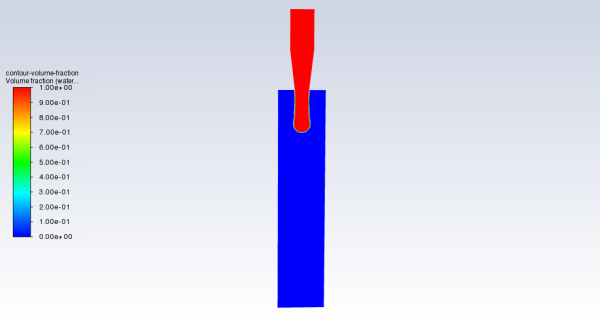
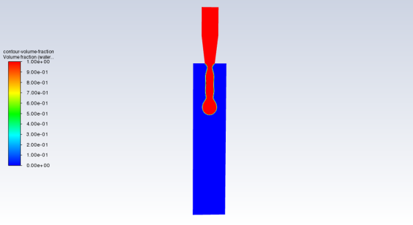
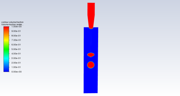
This tutorial demonstrated the application of the volume of fluid method with surface tension effects. The problem involved the 2D axisymmetric modeling of a transient liquid-gas interface, and postprocessing showed how the position and shape of the surface between the two immiscible fluids changed over time.