This tutorial is divided into the following sections:
This tutorial illustrates the setup and solution of a Selective Catalytic Reaction (SCR) system calculation using Ansys Fluent. The selective catalytic reduction of nitrogen oxides by injecting reducing agents has received increasing attention in the automotive industry for the removal of harmful gases. Ammonia is typically used as an agent to react with NOx in the presence of catalysts due to the lower exhaust temperature in the diesel engines.
However, to ensure safe and convenient storage and operation, the urea-water solution is often used in automobile after treatment systems. The urea-water solution is injected into the exhaust gas upstream of the SCR catalyst. The liquid jet goes through steps including liquid atomization, evaporation/decomposition and hydrolysis to form a mixture consisting of ammonia, iso-cyanic acid, water vapor, oxygen and other species. The mixture reacts with NOx in the SCR catalyst to reduce the NOx in the exhaust gas stream.
SCR performance is measured on the basis of its de-NOx efficiency, ammonia and iso-cyanic acid slip rates. These parameters heavily depend on the exhaust temperature, the NOx concentration, and the mixture quality at the catalyst inlet, which is mainly determined by the urea injection and decomposition rate.
Mesh file is provided with this tutorial, however the following points need to be considered while creating the geometry and meshing the volume.
Geometric Considerations:
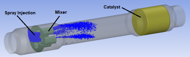
Computational domain consists of three parts:
Injector (spray development region).
Mixer.
Catalyst.
Separate fluid zone needs to be created for catalyst, because it is modelled as porous region.
In place of resolving insulation (mesh inside solid material), it can be modelled using thick-wall (shell-elements) approach.
Note: It is important to model insulation as it influences the wall temperature and hence urea deposition. Resolving the mesh in the insulation region will provide accurate result, but creating mesh in thin walls and insulation can be tedious and CPU intensive. A better approach is available where thermal behavior of insulation and thin metal is modeled with the shell conduction model. This model solves for thermal conduction both in the normal direction, as well as in the planar directions of the wall.
Mesh Considerations:
The following points were considered while meshing the volume:
Spray development region: Uniform mesh.
Boundary layer: 4 inflation layers adjacent to all walls.
This tutorial demonstrates how to do the following:
Use the porous medium model.
Use the laminar finite rate reaction model.
Set up a spray injection of a multicomponent droplet.
Model wall film using SCR specific impingement/splashing model.
Post process results to obtain SCR specific risk analysis evaluation.
This tutorial is written with the assumption that you have completed the introductory tutorials found in this manual and that you are familiar with the Ansys Fluent outline view and ribbon structure. Some steps in the setup and solution procedure will not be shown explicitly.
An automotive selective catalytic reduction system shown in Figure 20.1: Schematic of the selective catalytic reduction system will be modeled.
In this tutorial you will simulate the injection, liquid atomization, evaporation/decomposition, mixing, and wall film formation and evolution, that takes place inside the automotive SCR systems. To check the performance of the SCR system you will use:
The concept of uniformity index, which gives an indirect indication of the de–NOx efficiency of the SCR system. The area-weighted uniformity index of a specified field variable
 is defined as:
(20–1)
where
 is the area–weighted average value and A is the facet area.
SCR specific post–processing tools for assessing the risk for solids deposit formation.
The following sections describe the setup and solution steps for this tutorial:
- 20.4.1. Preparation
- 20.4.2. Reading and Checking the Mesh
- 20.4.3. General Settings
- 20.4.4. Solver Settings
- 20.4.5. Specifying the Models
- 20.4.6. Materials
- 20.4.7. Cell Zone Conditions
- 20.4.8. Specifying Boundary Conditions
- 20.4.9. Modify the Particle Properties
- 20.4.10. Flow Simulation
- 20.4.11. Postprocessing the Solution Results
To prepare for running this tutorial:
Download the
selective_catalytic_reduction.zipfile here .Unzip
selective_catalytic_reactor.zipto your working directory.The mesh file
scr_hexprism.msh.h5can be found in the folder.Use the Fluent Launcher to start Ansys Fluent.
Select Solution in the top-left selection list to start Fluent in Solution Mode.
Select 3D under Dimension.
Enable Double Precision under Options.
Set Solver Processes to
4under Parallel (Local Machine).Browse to the working directory in General Options tab and press Start button.
Read the mesh file
scr_hexprism.msh.h5. File → Read → Mesh...
Check the mesh.
Domain → Mesh
→ Check → Perform Mesh
CheckNote: Mesh check will perform various checks and will report the results in the console. Ensure that the reported minimum volume is positive
 .
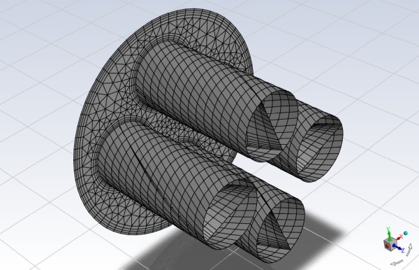
.The SCR geometric model is a long structure made of various cylindrical co-axial parts of different diameter, joined together by conical transitions. The inlet, outlet and central cylindrical parts have radius of 0.1 [m] and the two larger cylindrical parts have radius of 0.125 [m]; the upstream one contains the mixer, the downstream one the catalyst. The mixer is made of 3 zero–thickness surfaces: wall_mixer–pipes, wall_mixer–plate and wall_mixer–twisted and since they are internal walls, they appear as twins (for example,
wall_mixer–pipesandwall_mixer–pipes_shadow).Note: it’s good practice to display one surface at a time to visually confirm that all surfaces have the intended name. For this tutorial, follow this procedure to familiarize yourself with the model.
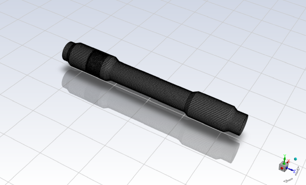
Examine the mesh.
Domain → Mesh
→ Display
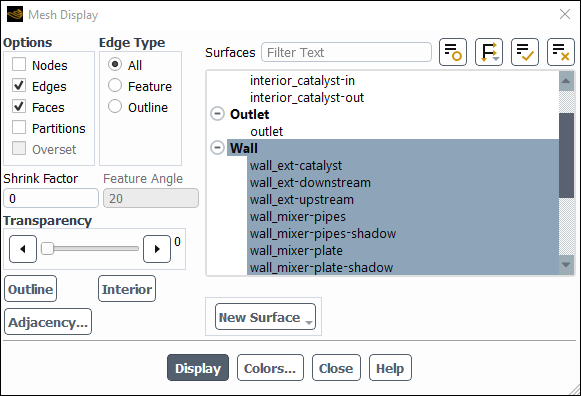
Select the Edges option and retain the default Faces option in the Options group box.
Deselect all surfaces an then select all the wall surfaces by selecting the Wall surface type.
Click
 to deselect all surfaces. Click
  and select Surface Type under
Group By to list the surfaces by type, as shown
above.
and select Surface Type under
Group By to list the surfaces by type, as shown
above.Click .
Rotate and adjust the magnification of the view.
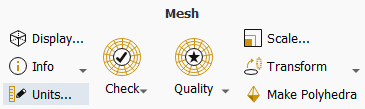
In the Mesh group box of the Domain ribbon tab, set the units for length..
![]() Domain → Mesh
→ Units...
Domain → Mesh
→ Units...
This opens the Set Units dialog box.
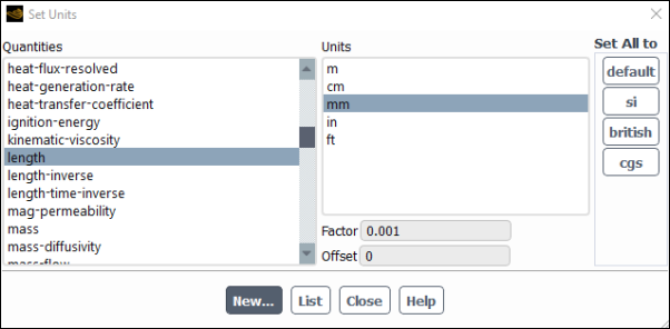
Select length under Quantities.
Select mm under Units.
Select Temperature under Quantities.
Select C under Units.
Close the Set Units dialog box.
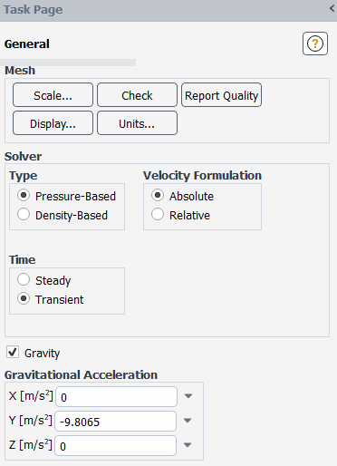
Enable the pressure-based steady solver including the effects of gravity.
Physics → Solver
→ General
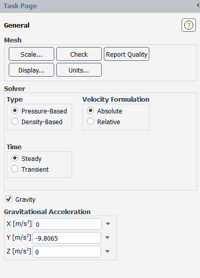
Retain the default selection of Pressure-Based from the Type list.
The pressure-based solver must be used for multiphase calculations.
Select Steady from the Time list.
Enable Gravity.
Enter
-9.8065m/s2 for the Gravitational Acceleration in the Y direction.
In this tutorial, the energy equation and the species conservation equations will be solved, along with the momentum and continuity equations.
You will use the default settings for the k-ω SST turbulence model, so you can enable it directly from the tree by right-clicking the Viscous node and choosing SST k-omega from the context menu.
 Setup → Models
→ Viscous
Setup → Models
→ Viscous  Model
→ SST k-omega
Model
→ SST k-omega
Enable chemical species transport and reaction.
Physics → Models
→ Species...
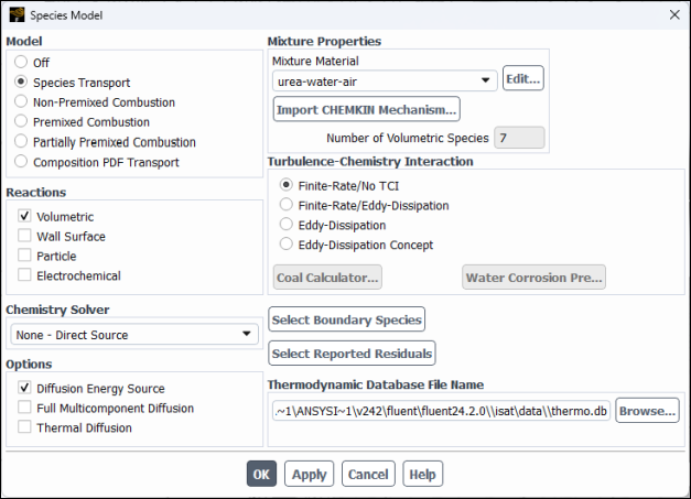
Select Species Transport in the Model list.
Enable Volumetric in the Reactions group box.
Ensure that Diffusion Energy Source is checked in the Options group box.
Select urea–water-air from the Mixture Material drop-down list.
Note: Assignment of Fluent library mixture material urea–water–air and the activation of volumetric reactions, loads a finite rate chemistry reaction mechanism with two gaseous reactions: CO(NH_2 )_2↔ NH_3+HCNO and HCNO+H_2 O↔ NH_3+CO_2. These species along with air (O2 and N2) are the 7 components of the mixture, shown in Number of Volumetric Species.
Click to close the Species Model dialog box.
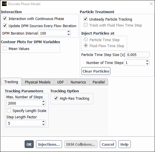
Enable Discrete Phase Model
Physics → Models
→ Discrete Phase...
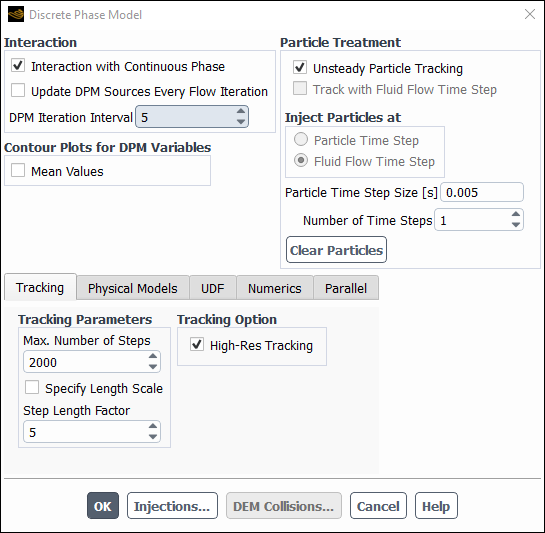
Enable the Interaction with Continuous Phase in the Interaction group box.
Note: This is required for the activation of unsteady particle tracking with steady state solver.
Set the DPM Iteration Interval to
5.Enable the Unsteady Particle Tracking in the Particle Treatment group box and change the value of Particle Time Step [s] to
0.005.Note: Although gas flow can be treated in a steady-state manner, the injection and motion of the droplets must be treated as transient.
Increase the Max. Number of Steps in Tracking Parameters group box to
2000.Ensure that the High-Res Tracking is enabled in the Tracking Option group box.
Click the Injections button.
Click the Create button.
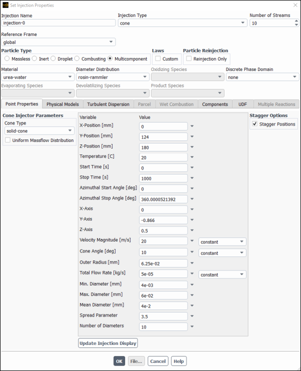
Select Cone as the Injection Type and set the Number of Streams to
10.Select Multicomponent as the Particle Type.
Select urea-water from the Material drop-down list.
Select rosin–rammler from the Diameter Distribution drop-down list.
Confirm solid-cone is selected in the Cone Type drop-down list at Cone Injector Parameters group box.
Set the X-Position [m] to
0mm, Y-Position [mm] to124mm, and the Z-Position [mm] to180mm.Set the Temperature [C] to
20C.Set the Start Time [s] to
0s and Stop Time [s] to1000sSet the Azimuthal Start Angle [deg] to
0degrees and the Azimuthal Stop Angle [deg] to360degrees.Set the X-Axis, Y-Axis and Z-Axis to
0,-0.866and0.5, respectively .Set the Velocity Magnitude [m/s] to
20m/s.Set the Cone Angle to
10degrees.Set the Outer Radius [mm] to
6.25e-02mm.Set the Total Flow Rate [Kg/s] to
5e-05Kg/sSet the Min. Diameter [mm] to
4e-03mm and the Max. Diameter [mm] to6e-02mm.Set the Mean Diameter [mm] to
4e-02mm.Set the Spread Parameter to
3.5.Set the Number of Diameters to
10.
Note: Start Time and Stop Time are given the above values for the tutorial purposes. For practical SCR applications these should be defined according to the actual urea dosing intervals.
In the tab
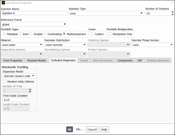
Select Discrete Random Walk Model.
Note: This makes sure that particles are not always injected with the same exactly parameters, rather they follow a stochastic behavior with average values as declared in the point properties table above and a perturbation that creates a more realistic turbulence representation.
In the tab
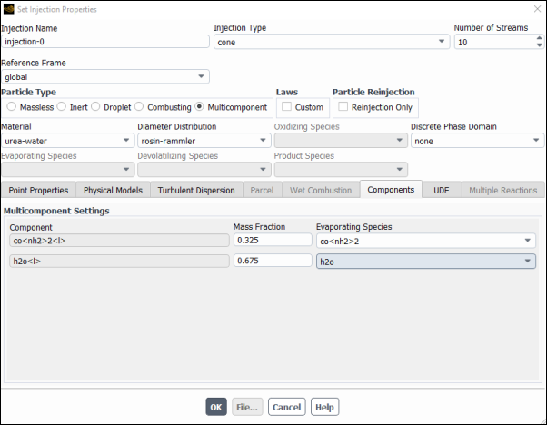
Select co<nh2>2 for the co<nh2>2<l> Component from the Evaporating Species drop–down list and enter
0.325for its Mass Fraction.Select h2o for the <h2o>2<l> Component from the Evaporating Species drop–down list and enter
0.675for its Mass Fraction.
Click to close the Set Injection Properties panel.
Click to close the Injections panel.
Click to close the Discrete Phase Model panel.
Create another injection by first copying the injection-0.
Setup →
Models → Discrete Phase
→ Injections → Injection-0
Copy...
This will create Injection-1 having the same properties as Injection-0. Change the Value of only the following Variable of Injection-1 in Point Properties tab.
Set the X-Position [m] to
4.48mm, Y-Position [mm] to123mm, and the Z-Position [mm] to172.707mm.Set the X-Axis to
0.15038.Set the Y-Axis to
-0.95511.Set the Z-Axis to
0.25523.Click to close the Set Injection Properties panel.
Repeat the procedure to create a third injection by copying injection–1.
Setup →
Models → Discrete Phase
→ Injections → Injection-1
Copy...
This will create Injection-2 having the same properties as Injection-1. Change the Value of only the following Variable of Injection-1 in Point Properties tab.
Set the X-Position to
-4.48mm.Set the X-Axis to
-0.15038.Click to close the Set Injection Properties panel.
Modify the material properties:
Confirm the properties for the mixture materials.
Setup → Materials
→ Mixture → urea-water-air
Edit...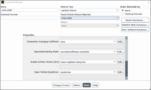
Click the button to the right of the Mixture Species drop-down list to open the Species dialog box. Confirm that the last of the 7 species on the list Selected Species is
n2.Then click to return to the dialog box.
Edit the particle mixture by selecting in the drop-down list. There is only one item in the drop-down list.
Select convection/diffusion-controlled for the Vaporization/Boiling Model.
Note: The convection/diffusion model is recommended for high evaporation rates.
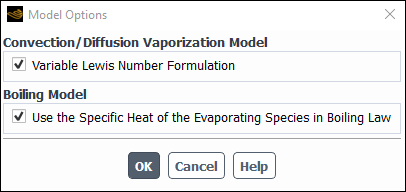
In the Model Options dialog box, enable Variable Lewis Number Formulation in Convection/Diffusion Vaporization Model. This causes the Use the Specific Heat of the Evaporating Species in Boiling Law in Boiling Model to be also enabled.
Note: Variable Lewis number allows Spalding heat transfer number and Spalding mass number to be different.
Click in the Model Options dialog box.
Click to accept the material property settings.
In the dialog box, Select press button and the dialog box will appear.
Select from the drop-down list and from the list.
Click and close the dialog box.
Close the Create/Edit Materials dialog box.
Set the cell zone conditions for the catalyst:![]() Setup
→ Cell Zone Conditions → Fluid
→ fluid_catalyst
Setup
→ Cell Zone Conditions → Fluid
→ fluid_catalyst
![]() Edit...
Edit...
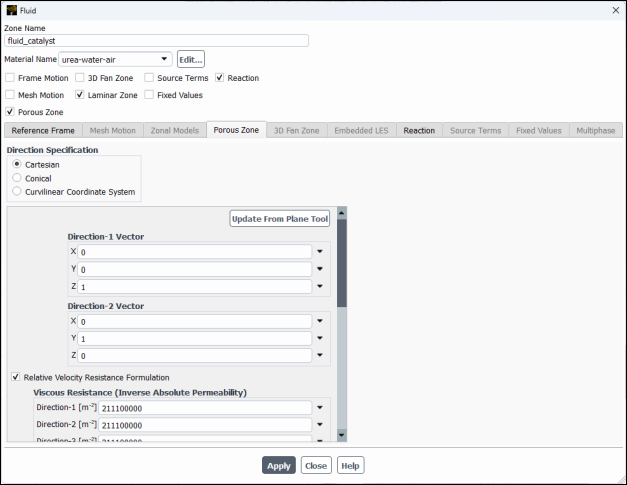
Enable Porous Zone to activate the porous zone model.
Enable Laminar Zone to solve the flow in the porous zone without turbulence.
Click the Porous Zone tab.
Make sure that the principal direction vectors are set as shown in Table 20.1: Values for the Principle Direction Vectors.
Ansys Fluent automatically calculates the third (Z direction) vector based on your inputs for the first two vectors. The direction vectors determine which axis the viscous and inertial resistance coefficients act upon.
Table 20.1: Values for the Principle Direction Vectors
Axis Direction-1 Vector Direction-2 Vector X 0 0 Y 0 1 Z 1 0 For the viscous and inertial resistance directions, enter the values in Table 20.2: Values for the Viscous and Inertial Resistance.
Scroll down to access the fields that are not initially visible.
Table 20.2: Values for the Viscous and Inertial Resistance
Direction Viscous Resistance (1/m2) Inertial Resistance (1/m) Direction-1 2e+07 10 Direction-2 2e+10 10000 Direction-3 2e+10 10000 Note: This setup provides a finite resistance to flow in the axial Z-direction and practically infinite resistance to the other two directions, therefore straightening the flow along the axial direction. The values of coefficients in Z-direction are estimated from the measured pressure losses along the catalyst, as a function of gases velocity, whereas the coefficients in the other two directions are typically taken to be three orders of magnitude larger.
Click and close the Fluid dialog box.
Set the boundary conditions of external wall wall_ext-catalyst.
Setup → Boundary
Conditions → Wall
→ wall_ext-catalyst
Edit...
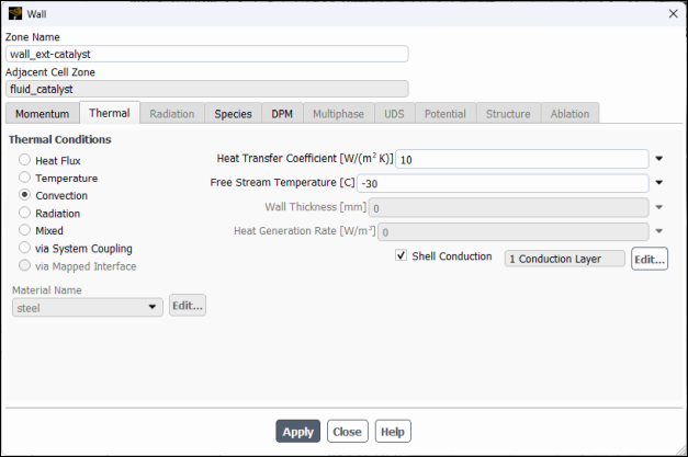
Click the Thermal tab.
Select Convection under Thermal Conditions and enter
10for the Heat Transfer Coefficient and-30for the Free Stream Temperature .Select under .
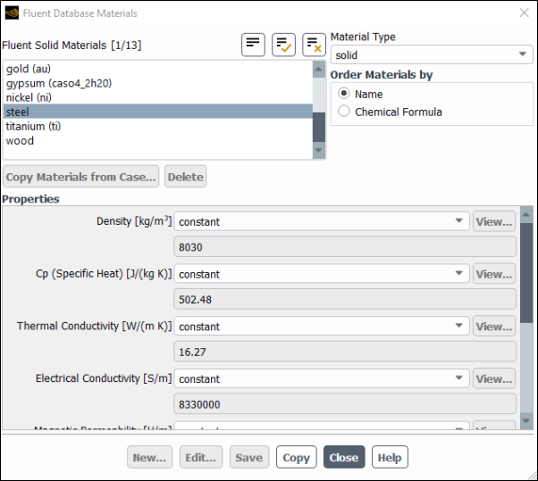
Enable Shell Conduction and then select Edit.
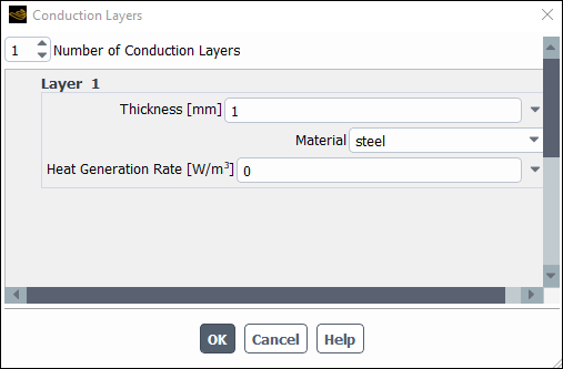
Enter
1mm for Thickness.Select
steelfrom the Material drop down list.Note: Shell conduction model allows to use zero–thickness walls, hence saving in mesh count, and simultaneously solve accurately conductive heat transfer inside solids not only along the thickness but also along the wall in both lateral directions, which is necessary in conductive materials such as metals. In case of temperature–dependent solid thermal conductivity and anticipated large variations in temperature, more than one shell layers maybe be necessary to accurately account for the in–thickness temperature distribution.
Click in the Conduction Layers dialog box.
Select Species tab and confirm that for all species have Specified Mass Flux is selected for the Species Boundary Condition and has a value of
0specified for the Species Mass Fraction/ Mass Flux.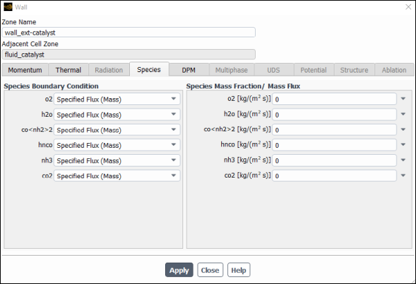
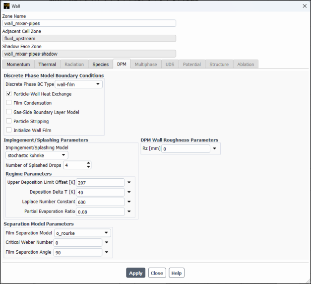
Select the DPM tab.
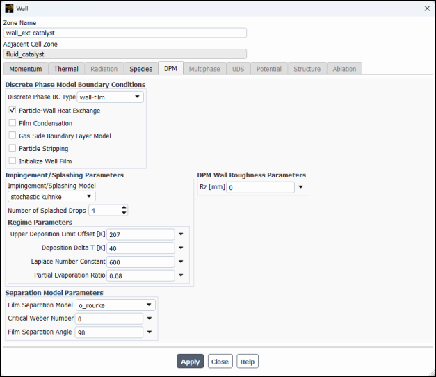
Select wall-film from the Discrete Phase BC Type drop–down list in the Discrete Phase Model Boundary Conditions group.
Enable Particle–Wall Heat Exchange.
Select
stochastic kuhnkefrom the Impingement/Splashing Model drop-down list in the Impingement/Splashing Parameters group box, retaining the default values.Note: Stochastic Kuhnke model is derived from the Kuhnke model and has been developed and calibrated for addressing SCR applications. It introduces stochastic effects into the critical temperature transition process, and the ʺpartial evaporationʺ concept for the evaporative splash regime.
Click and close the Wall dialog box.
Set the boundary conditions for internal wall wall_mixer–pipes.
Setup → Boundary
Conditions → Wall
→ wall_mixer–pipes
Edit...
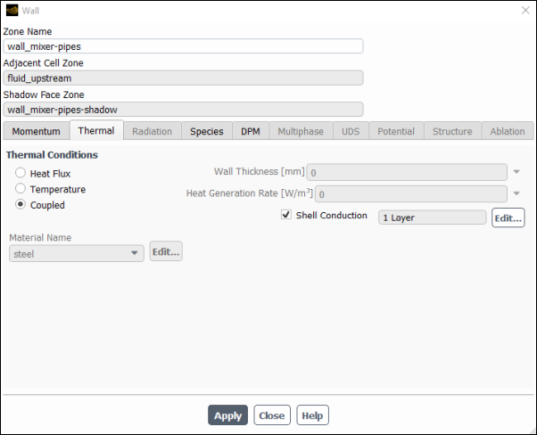
Click the Thermal tab.
Confirm that Coupled is selected in the Thermal Conditions group box.
Enable Shell Conduction and then select Edit.
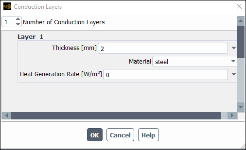
Enter
2mm for Thickness.Select
steelfrom the Material drop down list.Click in the Conduction Layers dialog box.
Select Species tab and confirm that for all species have Specified Mass Flux is selected for the Species Boundary Condition and has a value of
0specified for the Species Mass Fraction/ Mass Flux.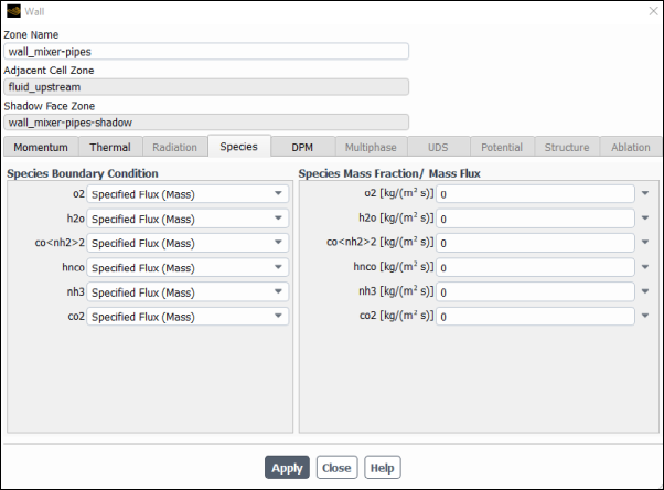
Select the DPM tab.
Select wall-film from the Discrete Phase BC Type drop–down list in the Discrete Phase Model Boundary Conditions group.
Enable Particle–Wall Heat Exchange.
Select
stochastic kuhnkefrom the Impingement/Splashing Model drop-down list in the Impingement/Splashing Parameters group box, retaining the default values.
Click and close the Wall dialog box.
Copy the boundary conditions to the other external walls.
Setup → Boundary
Conditions → Wall
→ wall_ext-catalyst
Copy...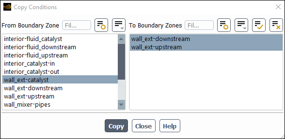
Ensure that wall_ext–catalyst is selected from the From Boundary Zone list.
Select all the walls from the To Boundary Zone list.
Click Copy, click OK in the confirmation prompt, and close the Copy Conditions dialog box.
Copy the boundary conditions to the other internal walls.
Setup → Boundary
Conditions → Wall
→ wall_mixer-pipes
Copy...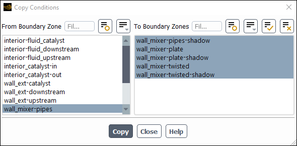
Ensure that wall_mixer-pipes is selected from the From Boundary Zone list.
Select all the walls from the To Boundary Zone list.
Click Copy, click OK in the confirmation prompt, and close the Copy Conditions dialog box.
Set the boundary conditions for the inlet, first change its type from velocity-inlet to mass-flow-inlet.
Setup → Boundary
Conditions → Inlet
→ inlet Type → mass-flow-inlet
Set the conditions for mass-flow-inlet.
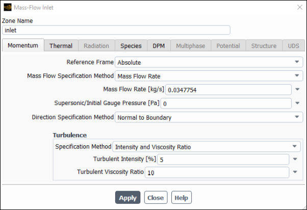
Enter
0.0347754kg/s for Mass Flow Rate .Click the Thermal tab and enter
400C for Total Temperature.Click the Species tab, set the Species Mass Fractions for o2 to
0.001, h2o to0.08, and co2 to0.02.Click the DPM tab and confirm that escape is selected for Discrete Phase BC Type.
Click and close the Mass Flow Inlet dialog box.
Set the boundary conditions for outlet.
Setup → Boundary
Conditions → Outlet
→ outlet Edit...
Click the Thermal tab, enter
400C for Temperature.Click the Species tab, set all the Backflow Species Mass Fractions to
0.Click the DPM tab and confirm that escape is selected for Discrete Phase BC Type.
Click and close the Pressure Oulet dialog box.
Thermolysis model applies for both the free particles and wall film. Since wall film is now activated in the boundary conditions thermolysis can now be setup in the materials. Modify the material properties:
Select secondary rate for Thermolysis of particles and wall film:
Setup → Materials
→ Particle Mixture
→ urea–water → urea-liquid
Edit...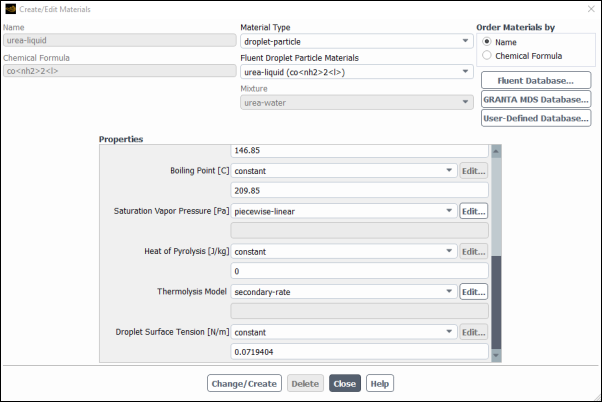
Select for the .
Note: Secondary rate thermolysis model allows to define different thermolysis parameters for the particles and film.
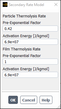
Enter
1.0for the in group box.Click to close the dialog box.
Click to accept the material property settings.
Close the Create/Edit Materials dialog box.
Specify the discretization schemes.
Solution → Solution
→ Methods...
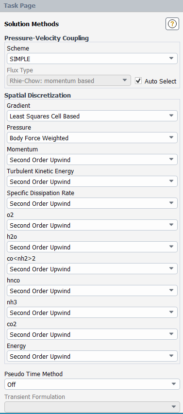
Select SIMPLE from the Pressure-Velocity Coupling drop-down list.
Enable Auto Select for the Flux Type.
Select Body Force Weighted for Pressure, Second Order Upwind for Momentum, Energy and all the Species in the Spatial Discretization group box.
Set the solution control parameters.
Solution → Solution
→ Controls...
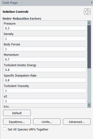
Retain the default Under Relaxation Factors for all variables.
Click to open the dialog box.

Enter
-50C for the Minimum Static Temperature.Enter
700C for the Maximum Static Temperature.Click to close the Solution Limits dialog box.
Note: It's good practice to limit the allowable range of temperature (and/or pressure in other cases) to avoid stability problems.
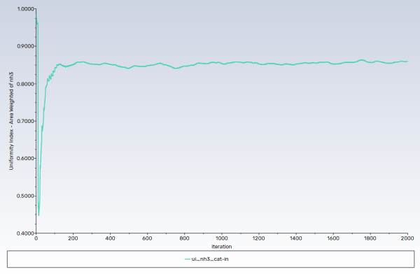
Create a surface report definition of the species at the interior catalyst.
Solution → Reports
→ Definitions → New
→ Surface Report → Uniformity
Index-Area Weighted...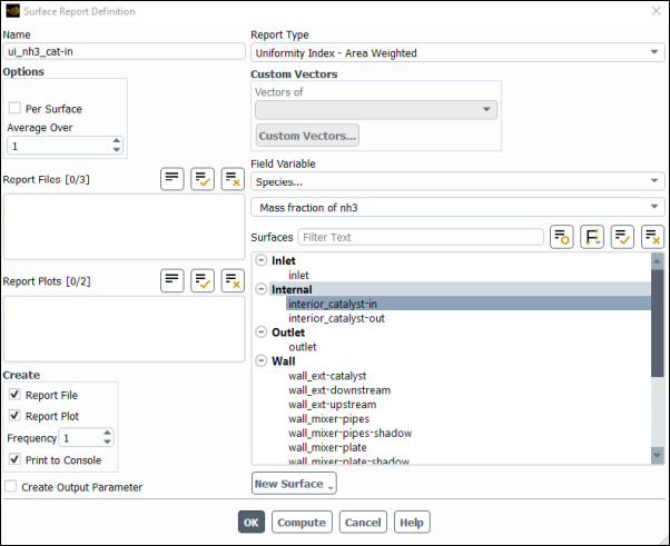
Enter
ui_nh3_cat-infor the Name of the report definition.Enable Report File, Report Plot, and Print to Console in the Create group box.
Select Species... and Mass fraction of nh3 from the Field Variable drop-down lists.
Select interior_catalyst-in from the Surfaces selection list.
Click to save the surface report definition and close the Surface Report Definition dialog box.
Create a surface report definition of the velocity at the interior catalyst.
Solution → Reports
→ Definitions → New
→ Surface Report → Uniformity
Index-Area Weighted...
Enter
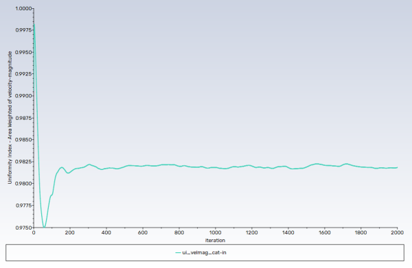
ui_velmag_cat-infor the Name of the report definition.Enable Report File and Report Plot in the Create group box.
Select Velocity... and Velocity Magnitude from the Field Variable drop-down lists.
Select interior_catalyst-in from the Surfaces selection list.
Click to save the surface report definition and close the Surface Report Definition dialog box.
Create a surface report definition of the wall film mass.
Solution → Reports
→ Definitions → New
→ Surface Report
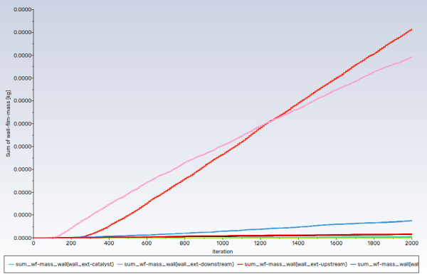
→ Sum...Enter
sum_wf-mass_wallsfor the Name of the report definition.Enable separate reporting for each surface by checking Per Surface box in the Options group box.
Enable Report File and Report Plot in the Create group box.
Select Wall Film... and Wall Film Mass from the Field Variable drop-down lists.
Select all the walls from the Surfaces selection list.
Click to save the surface report definition and close the Surface Report Definition dialog box.
Initialize the flow field using the Initialization group box of the Solution ribbon tab.
Solution → Initialization
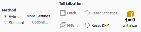
Retain the default selection of Hybrid from the Method list.
Click .
Save the case and dat file (
scr_initial.cas.h5andscr_initial.dat.h5.) File → Write →
Case & Data...
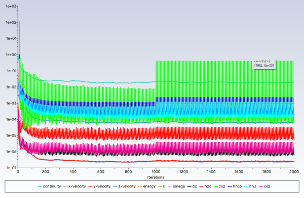
Request 2000 iterations.
Solution → Run Calculation
→ Calculate
Note: Convergence in this case is not judged by the residuals, rather from the monitors. Both uniformity monitors show that main phase (gases) flow has been stabilized, whereas the wall film mass monitor suggests, as expected, that disperse phase flow (droplets and wall film) is developing.
Save the case and dat file (
scr_solved.cas.h5andscr_solved.dat.h5.) File → Write →
Case & Data...
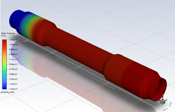
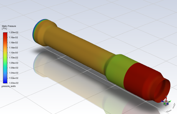
Display contours of pressure.
Results → Graphics
→ Contours → New...
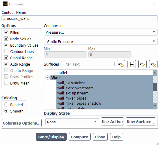
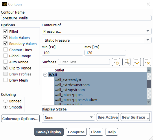
Enter
pressure_wallsfor Contour Name.Select Pressure... and Static Pressure from the Contours of drop-down lists.
Select Wall from the Surfaces selection list.
Click .
Contours show that static pressure drops from ~112 to ~2 [Pa] across the catalyst.
Create two longitudinal planes to plot variables at the SCR internal region. These two surfaces will be used to display solution results internally the SCR system.
Create a surface of constant x.
Results → Surface
→ Create →
Iso-Surface...
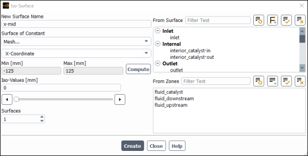
Enter
x-midfor New Surface Name.Select Mesh... and X-Coordinate from the Surface of Constant drop-down lists.
Click .
The Min and Max fields display the x-extent of the domain.
Retain a value of
0mm for Iso-Values.Click and close the Iso-Surface dialog box.
Repeat steps above and create a surface of constant y.
Results → Surface
→ Create →
Iso-Surface...
Enter
y-midfor New Surface Name.Select Mesh... and Y-Coordinate from the Surface of Constant drop-down lists.
Click .
The Min and Max fields display the x-extent of the domain.
Retain a value of
0mm for Iso-Values.Click and close the Iso-Surface dialog box.
Display the mesh surfaces.
Results → Graphics
→ Mesh → New...
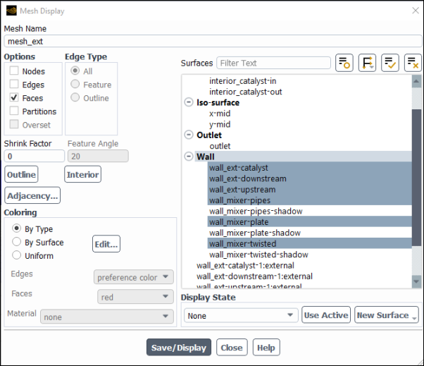
Enter
mesh_extfor Mesh Name.Confirm that only Faces have been selected in the Options group box.
Select all the Wall surfaces, except those with suffix
-shadow. This is to avoid plotting twice the internal (double) walls.Click and close the Mesh Display dialog box.
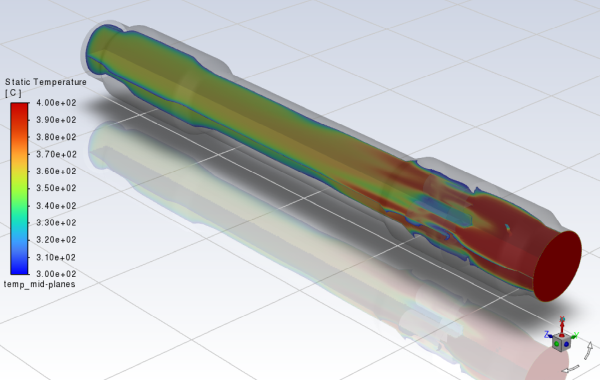
Display contours of gas temperature field inside the SCR with the geometry also displayed.
Results → Graphics
→ Contours → New...
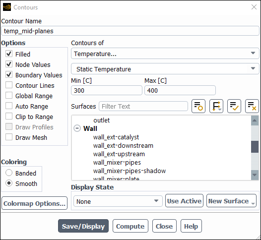
Enter
temp_mid-planesfor Contour Name.Disable Global Range, Auto Range and Clip to Range in the Options group box.
Select Temperature... and Static Temperature from the Contours of drop-down lists.
Change the Min value to
300C.Change the Max value to
400C.Select Inlet,Outlet and Iso-surface from the Surfaces selection list.
Click and close the Contours dialog box.
Create a scene containing the static temperature distribution at the two internal surfaces.
Results → Scene
New...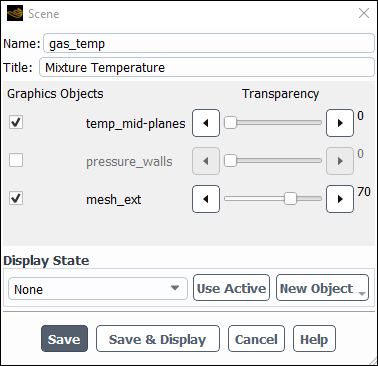
Change the Name to
gas_temp.Change the Title to
Mixture Temperature.Enable the mesh_ext and temperature_mid–planes graphics object.
Set the Transparency of mesh_ext object to 70.
Click and close the Scene dialog box.
The gases enter the domain at 400 [C] but when mixed with the cooler droplets (at 20 [C]) and also due to droplets partial evaporation, they are cooled down to an average temperature of ~315 [C] at the outlet. Note that values below the minimum and above the maximum values set in the contour dialog box, are displayed as blue and red, respectively, due to deactivation of option, otherwise they would have been displayed as empty regions.
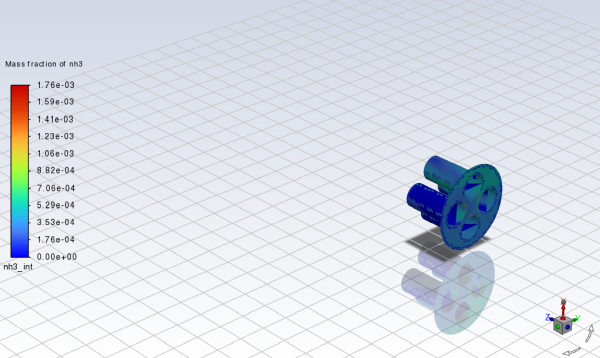
Create a contour of NH3 distribution on the mixer
Results → Graphics
→ Contours → New...
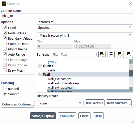
Enter
nh3_intfor Contour Name.Disable Global Range in the Options group box.
Select Species... and Mass fraction of nh3 from the Contours of drop-down lists.
Select all internal walls from the Surfaces selection list.
Click and close the Contours dialog box.
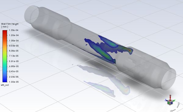
Display contours of Wall Film Height.
Results → Graphics
→ Contours → New...
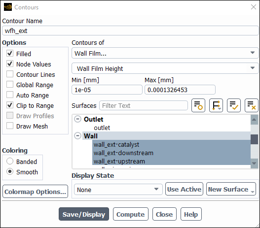
Enter
wfh_extfor Contour Name.Disable Global Range and Auto Range in the Options group box.
Select Wall Film... and Wall Film Height from the Contours of drop-down lists.
Select the external walls from the Surfaces selection list.
Click Compute.
Ensure that Clip to Range is selected in the Options group box.
Change the Min value to
1e-05mm.Click and close the Contours dialog box.
Create a scene with the wall film height distribution on all walls.
Results → Scene
New...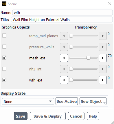
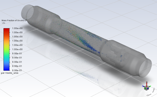
Create a particle tracks graph.
Results → Graphics
→ Particle Tracks
→ New...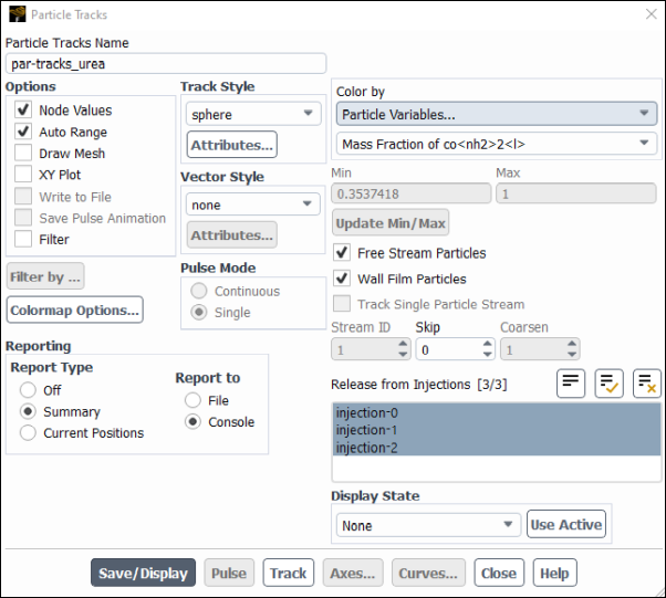
Enter
par-tracks_ureafor Particle Tracks Name.Select Sphere in the Track Style group box.
Click Attributes... and change the Scale to 100.
Click Apply and close the Particle Sphere Style Attributes dialogue box.
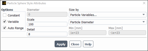
This will cause the particles to appear as spheres with a size proportional to their diameter and scaled by x100 for clarity.
Select Particle Variables... and Mass Fraction of co<nh2>2<l> from the Color by drop-down lists.
Select all three injections from the Release from Injections selection list.
Select Summary in the Reporting group box, so that both a summary in the console and a graph in the GUI will be produced.
Make sure that both Free Stream Particles and Wall Film Particles are checked.
Click .
Close the Particle Tracks dialog box.
The summary track report provides information about the number of particles in the domain, their fate (ʺevaporatedʺ, ʺtransformedʺ, ʺescapedʺ), their state (ʺIn Filmʺ, ʺIn Fluidʺ) and the associated mass and heat transfer, as well as their composition.
Create a scene with the particle tracks and the walls of the geometry.
Results → Scene
New...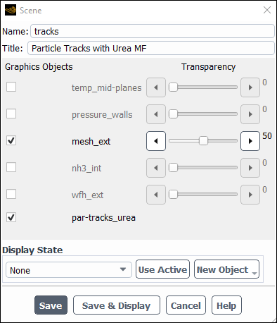
Change the Name to
tracks.Change the Title to
Particle Tracks with Urea MF.Enable the mesh_ext and par-tracks_urea graphics object.
Set the Transparency of mesh_ext object to 50.
Click and close the Scene dialog box.
Figure 20.13: Tracks of Free and Wall Film Particles, Colored by Urea Mass Fraction and Scaled by Particle Diameter.
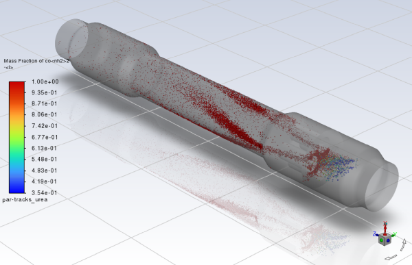
The particle track graph shows both the cloud of free droplets, as well as the wall particles that form the wall film. It is evident that water content of the droplets is evaporated upstream the mixer and is associated with the cooling effect observed in the gas temperature contour plot previously.
Modify the particles tracks to show only the wall film particles that have lost practically all their water content.
Results → Graphics
→ Particle Tracks
→ par-tracks_urea Edit..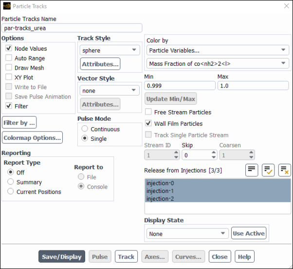
Uncheck Auto Range to be able to manually set the range of the plotted value.
Select Off in the Reporting group box.
Uncheck Free Stream Particles to hide them from the display.
Set the Min value to
0.999and the Max value to1.0, which practically means that all water content of the droplet has evaporated.Check the Filter option.
Select Filter By... to regulate filtering.
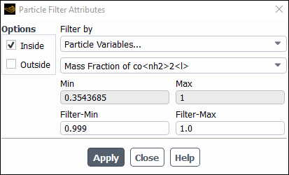
Select Particle Variables... and Mass Fraction of co<nh2>2<l> from the Filter By... drop-down lists.
Set the Filter-Min value to
0.999and Filter-Max value to1.0and make sure the remaining settings are as displayed.Click and close the Particle Filter Attributes dialog box.
Click and close the Particle Tracks dialog box.
Re-display the scene with the particle tracks and the walls of the geometry.
Results
→ Scene → tracks
Edit...Save the case and data files (
scr_final.cas.h5andscr_final.dat.h5). File → Write → Case & Data...
Ansys Fluent has an automated workflow to post process CFD results and assess the risk for solids deposit formation for SCR systems operating with urea. The calculations involve chemical and hydrodynamic risk factors based on thermodynamic data and known chemical pathways, as well as on experimental evidence reported. The risk variables are defined as dimensionless quantities that vary from 0 (no risk) to 1 (max risk). Note that the risk assessment calculation is not a predictive model for urea deposit formation, and the obtained results should be considered only as rough guidance in exploring urea deposit formation trends. The risk assessment calculation is invoked after initial film formation on SCR surfaces and requires the transient solver.
In the Solver group box of the Physics ribbon tab, select transient.
Physics → Solver →
General...
Modify the iterations interval between DPM tracks.
Physics → Models
→ Discrete Phase...
Change the DPM Iteration Interval to
100.By setting a value equal or larger than the maximum number of iterations per time step, the particle tracking is only performed once per time step.
Click to close the Discrete Phase Model panel.
Activate the urea risk assessment from the TUI.
Press
Enterin the console to get the command prompt (>).Type
/define/models/dpm/options/scr-urea-deposition-risk-analysis
                enable?
Type
yesin the console and press <Enter>.Type all IDs (provided in the Boundary Conditions list on the model tree) one by one followed by
Enter. When the last wall ID has been typed, pressEnteragain. You should get the following output in the console./define/models/dpm/options/scr-urea-deposition-risk-analysis> enableEnable the SCR urea deposition risk analysis? [no] y Wall face zones(1) [()] 4 Wall face zones(2) [()] 5 Wall face zones(3) [()] 6 Wall face zones(4) [()] 9 Wall face zones(5) [()] 10 Wall face zones(6) [()] 16 Wall face zones(7) [()] 17 Wall face zones(8) [()] 18 Wall face zones(9) [()] 19 Wall face zones(10) [()]Fluent has also activated the in the Run Calculation Task Page. If is pressed the details can be seen.
Run the calculation.
Solution → Run Calculation
→ Run Calculation...
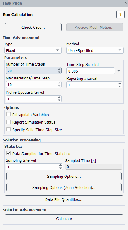
Enter
20for Number of Time Steps. This is a small time period covered, in order to demonstrate the procedure. Larger time periods may be simulated in industrial risk assessment calculations.Ensure that the Time Step Size to
0.005.Enter
10for Max Iterations/Time Steps. A transient simulation that converges every time step in 10 iterations or less is generally considered to have a sufficiently fine time step size.Click .
Fluent asks if the existing Report files will be over-written or new ones will be created. This happens because now the reports are not monitored every iteration (steady-state solver) but every time step (transient solver). Press to create new files. Fluent starts the transient calculation using the steady-state solution as the initial state of the transient solution. Residuals show that standard convergence is achieved in 10 iterations for all time steps (except a couple of steps at the beginning), which was expected as the steady-state gas flow was quite stable.
Examine the risk levels.
Results → Graphics
→ Contours → New...
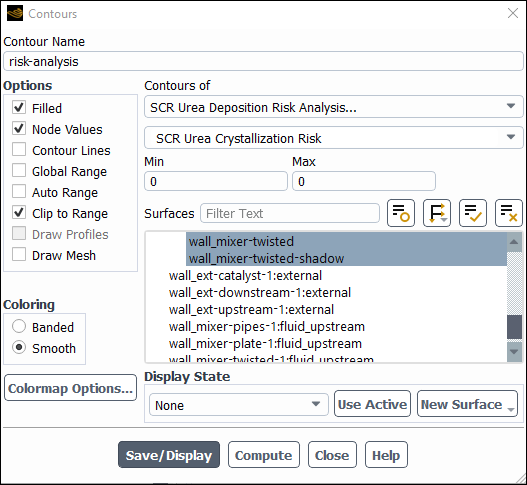
Enter
risk-analysisfor Contour Name.Disable Global Range and Auto Range in the Options group box.
Select SCR Urea Deposition Risk Analysis... and SCR Urea Crystallization Risk from the Contours of drop-down lists.
Select all walls from the Surfaces selection list.
Click Compute. Fluent returns
0for Min and Max, indicating that risk for crystallization is zero at all walls.Repeat the same for the other two risk parameters, SCR Urea Secondary Reactions Risk and SCR Overall Urea Chemical Deposition Risk, which also return zero risk everywhere.
Note: Risk assessment for solids deposition in urea SCR systems is based on empirical correlations using parameters reported in the relevant literature. The user can set the values of 9 such parameters through the TUI, according to the specific characteristics of the SCR system simulated.
Click and close the Contours dialog box.
Modify minimum mass fraction of HNCO from the TUI.
Press
Enterin the console to get the command prompt (>).Type
/define/models/dpm/options/scr-urea-deposition-risk-analysis
                seco-rx-min-hnco
in the console and pressEnter./define/models/dpm/options/scr-urea-deposition-risk-analysis> seco-rx-min-hncominimum HNCO mass fraction in the gas phase above the film for secondary reactions [0.03] 0.001Type
0.001in the console and pressEnter.
Continue the calculation for another 20 time steps
Re-examine the risk levels.
Results → Graphics
→ Contours → risk-analysis
Edit...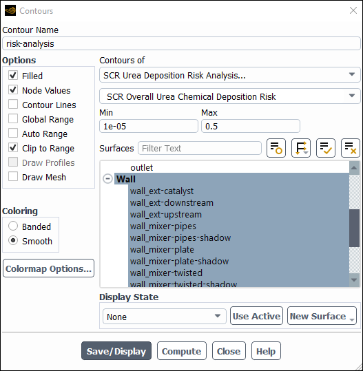
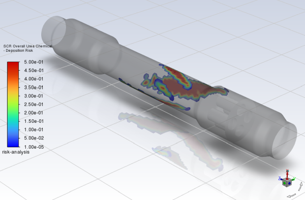
Select SCR Urea Deposition Risk Analysis... and SCR Overall Urea Chemical Deposition Risk from the Contours of drop-down lists.
Select all walls from the Surfaces selection list.
Click Compute and Fluent will return Min and Max values of
0and0.5, respectively.Set the Min value to
1e-05.Click and close the Contours dialog box.
Create a scene with the overall deposition risk and the walls of the geometry.
Results → Scene
New...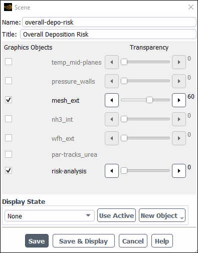
Save the case and data files (
scr_transient.cas.h5andscr_transient.dat.h5). File → Write →
Case & Data...