Chapter 23: Modeling Cavitation

This tutorial is divided into the following sections:

23.1. Introduction

This tutorial examines the pressure-driven cavitating flow of water through a sharp-edged orifice. This is a typical configuration in fuel injectors, and brings a challenge to the physics and numerics of cavitation models because of the high pressure differentials involved and the high ratio of liquid to vapor density. Using the multiphase modeling capability of Ansys Fluent, you will be able to predict the strong cavitation near the orifice after flow separation at a sharp edge.

This tutorial demonstrates how to do the following:

Set boundary conditions for internal flow.
Use the mixture model with cavitation effects.
Calculate a solution using the pressure-based coupled solver.

23.2. Prerequisites

This tutorial is written with the assumption that you have completed the introductory tutorials found in this manual and that you are familiar with the Ansys Fluent outline view and ribbon structure. Some steps in the setup and solution procedure will not be shown explicitly.

23.3. Problem Description

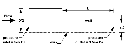
The problem considers the cavitation caused by the flow separation after a sharp-edged orifice. The flow is pressure driven, with an inlet pressure of 5 x 10⁵ Pa and an outlet pressure of 9.5 x 10⁴ Pa. The orifice diameter is 4 x 10^–3 m, and the geometrical parameters of the orifice are D/d = 2.88 and L/d = 4, where D, d, and L are the inlet diameter, orifice diameter, and orifice length respectively. The geometry of the orifice is shown in Figure 23.1: Problem Schematic.

Figure 23.1: Problem Schematic

23.4. Setup and Solution

The following sections describe the setup and solution steps for this tutorial:

23.4.1. Preparation

To prepare for running this tutorial:

Download the cavitation.zip file here .
Unzip cavitation.zip to your working directory.
The mesh file cav.msh can be found in the folder.
Use the Fluent Launcher to start Ansys Fluent.
Select Solution in the top-left selection list to start Fluent in Solution Mode.
Select 2D under Dimension.
Enable Double Precision under Options.

Note: The double precision solver is recommended for modeling multiphase flows simulation.
Set Solver Processes to 1 under Parallel (Local Machine).

23.4.2. Reading and Checking the Mesh

Read the mesh file cav.msh.
File → Read → Mesh...
Check the mesh.
Domain → Mesh → Check → Perform Mesh Check
Check the mesh scale.
Domain → Mesh → Scale...
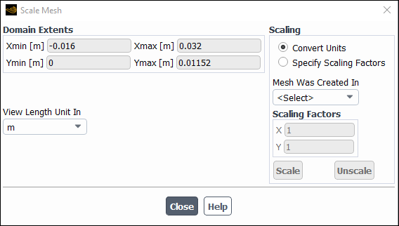
1. Retain the default settings.
2. Close the Scale Mesh dialog box.
Examine the mesh (Figure 23.2: The Mesh in the Orifice).
Figure 23.2: The Mesh in the Orifice

As seen in Figure 23.2: The Mesh in the Orifice, half of the problem geometry is modeled, with an axis boundary (consisting of two separate lines) at the centerline. The quadrilateral mesh is slightly graded in the plenum to be finer toward the orifice. In the orifice, the mesh is uniform with aspect ratios close to , as the flow is expected to exhibit two-dimensional gradients.
When you display data graphically in a later step, you will mirror the view across the centerline to obtain a more realistic view of the model.
Since the bubbles are small and the flow is high speed, gravity effects can be neglected and the problem can be reduced to axisymmetrical. If gravity could not be neglected and the direction of gravity were not coincident with the geometrical axis of symmetry, you would have to solve a 3D problem.

23.4.3. Solver Settings

Specify an axisymmetric model.
Setup → General
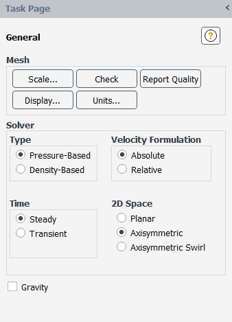
1. Retain the default selection of Pressure-Based in the Type list.
  The pressure-based solver must be used for multiphase calculations.
2. Select Axisymmetric in the 2D Space list.
Note: A computationally intensive, transient calculation is necessary to accurately simulate the irregular cyclic process of bubble formation, growth, filling by water jet re-entry, and break-off. In this tutorial, you will perform a steady-state calculation to simulate the presence of vapor in the separation region in the time-averaged flow.

23.4.4. Models

Enable the multiphase mixture model.
Physics → Models → Multiphase...
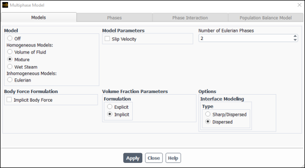
1. Select Mixture in the Model list.
  The Multiphase Model dialog box will expand.
2. Clear Slip Velocity in the Mixture Parameters group box.
  In this flow, the high level of turbulence does not allow large bubble growth, so gravity is not important. It is also assumed that the bubbles have same velocity as the liquid. Therefore, there is no need to solve for the slip velocity.
3. Click Apply and close the Multiphase Model dialog box.
  Important: When setting up your case, if you have made changes in the current tab, you should click the Apply button to make them effective before moving to the next tab. Otherwise, the relevant models may not be available in the other tabs, and your settings may be lost.
Enable the k-ω SST turbulence model.
Physics → Models → Viscous...
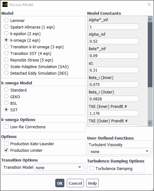
1. Retain the default selection of k-omega (2 eqn) in the Model list.
2. Retain the default selection of SST in the k-omega Model list
3. Click OK to close the Viscous Model dialog box.

23.4.5. Materials

For the purposes of this tutorial, you will be modeling the liquid and vapor phases as incompressible. Note that more comprehensive models are available for the densities of these phases, and could be used to more fully capture the affects of the pressure changes in this problem.

Create a new material to be used for the primary phase.
Setup → Materials → Fluid New...
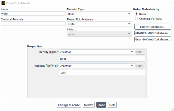
1. Enter water for Name.
2. Enter 1000 kg/m³ for Density.
3. Enter 0.001 kg/m–s for Viscosity.
4. Click Change/Create and select Yes.
Copy water vapor from the materials database and modify the properties of your local copy.
1. In the Create/Edit Materials dialog box, click the Fluent Database... button to open the Fluent Database Materials dialog box.
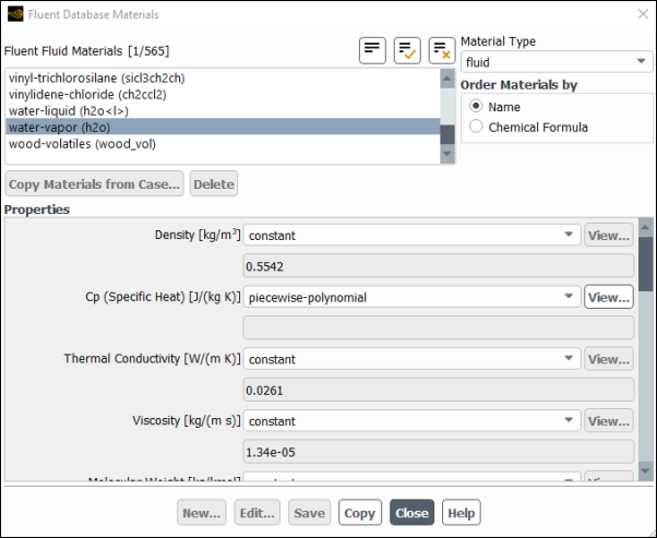
  1. Select water-vapor (h2o) from the Fluent Fluid Materials selection list.
    Scroll down the list to find water-vapor (h2o).
  2. Click Copy to include water vapor in your model.
    water-vapor appears under Fluid in the Materials task page
  3. Close the Fluent Database Materials dialog box.
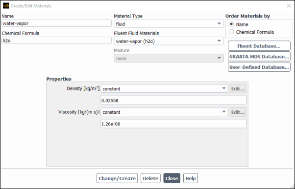
2. Enter 0.02558 kg/m³ for Density.
3. Enter 1.26e-06 kg/m–s for Viscosity.
4. Click Change/Create and close the Create/Edit Materials dialog box.

23.4.6. Phases

Setup → Models → Multiphase Edit...

In the Multiphase Model dialog box, go to the Phases tab.

Specify liquid water as the primary phase.
1. In the Phases selection list, select phase-1 – Primary Phase.
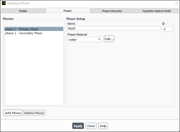
2. Enter liquid for Name.
3. Select water from the Phase Material drop-down list.
4. Click Apply.
Specify water vapor as the secondary phase.
1. In the Phases selection list, select phase-2 – Secondary Phase.
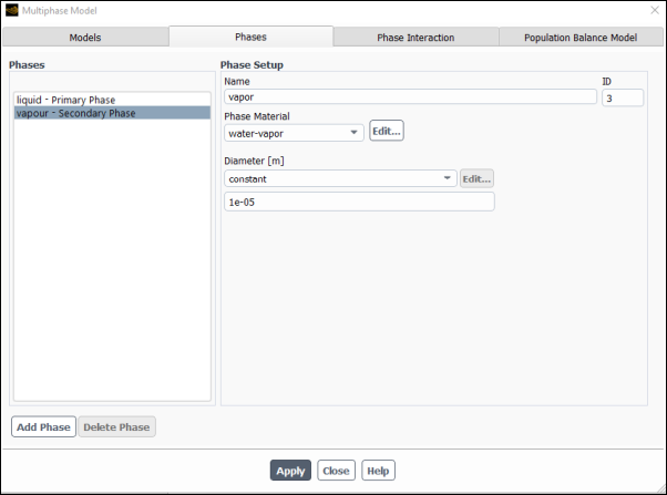
2. Enter vapor for Name.
3. Select water-vapor from the Phase Material drop-down list.
4. Click Apply.
Enable the cavitation model.
1. In the Multiphase Model dialog box, go to the Phase Interaction tab.
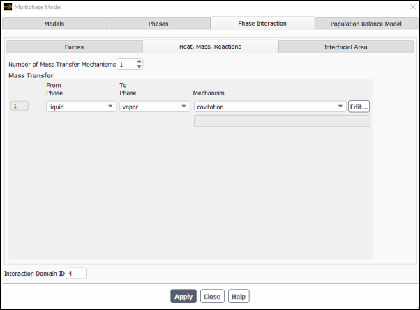
2. In the Heat, Mass, Reaction tab, set Number of Mass Transfer Mechanisms to 1.
  The dialog box expands to show relevant modeling parameters.
3. Ensure that liquid is selected from the From Phase drop-down list in the Mass Transfer group box.
4. Select vapor from the To Phase drop-down list.
5. Select cavitation from the Mechanism drop-down list.
  The Cavitation Model dialog box will open to show the cavitation inputs.
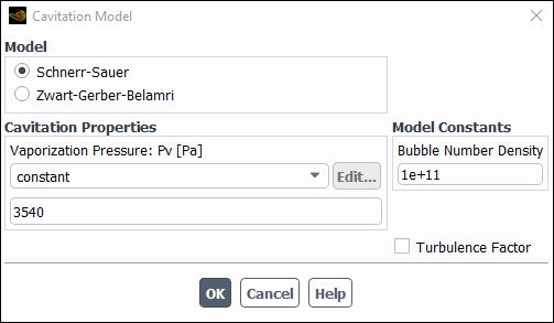
  1. Retain the value of 3540 Pa for Vaporization Pressure.
    The vaporization pressure is a property of the working liquid, which depends mainly on the temperature and pressure. The default value is the vaporization pressure of water at 1 atmosphere and a temperature of 300 K.
  2. Retain the value of 1e+11 for Bubble Number Density.
  3. Click OK to close the Cavitation Model dialog box.
6. Click Apply and close the Multiphase Model dialog box.

23.4.7. Boundary Conditions

For the multiphase mixture model, you will specify conditions for the mixture (that is, conditions that apply to all phases) and the conditions that are specific to the primary and secondary phases. In this tutorial, boundary conditions are required only for the mixture and secondary phase of two boundaries: the pressure inlet (consisting of two boundary zones) and the pressure outlet. The pressure outlet is the downstream boundary, opposite the pressure inlets.

Setup → Boundary Conditions

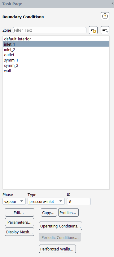
Set the boundary conditions at inlet_1 for the mixture. Ensure that mixture is selected from the Phase drop-down list in the Boundary Conditions task page.
Setup → Boundary Conditions → inlet_1 → Edit...
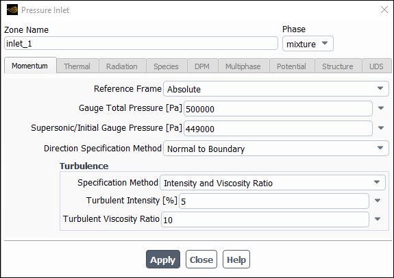
1. Enter 500000 Pa for Gauge Total Pressure.
2. Enter 449000 Pa for Supersonic/Initial Gauge Pressure.
  If you choose to initialize the solution based on the pressure-inlet conditions, the Supersonic/Initial Gauge Pressure will be used in conjunction with the specified stagnation pressure (the Gauge Total Pressure) to compute initial values according to the isentropic relations (for compressible flow) or Bernoulli’s equation (for incompressible flow). Otherwise, in an incompressible flow calculation, Ansys Fluent will ignore the Supersonic/Initial Gauge Pressure input.
3. Retain the default selection of Normal to Boundary from the Direction Specification Method drop-down list.
4. Retain the default settings in the Turbulence group box.
5. Click Apply and close the Pressure Inlet dialog box.
Set the boundary conditions at inlet_1 for the secondary phase.
Setup → Boundary Conditions → inlet_1
1. Select vapor from the Phase drop-down list.
2. Click Edit... to open the Pressure Inlet dialog box.
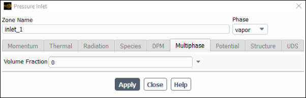
  1. In the Multiphase tab, retain the default value of 0 for Volume Fraction.
  2. Click Apply and close the Pressure Inlet dialog box.
Copy the boundary conditions defined for the first pressure inlet zone (inlet_1) to the second pressure inlet zone (inlet_2).
Setup → Boundary Conditions → inlet_1
1. Select mixture from the Phase drop-down list.
2. Click Copy... to open the Copy Conditions dialog box.
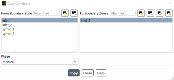
  1. Select inlet_1 from the From Boundary Zone selection list.
  2. Select inlet_2 from the To Boundary Zones selection list.
  3. Click Copy.
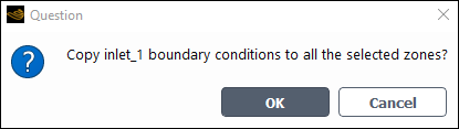
    A Question dialog box will open, asking if you want to copy inlet_1 boundary conditions to inlet_2. Click OK.
  4. Close the Copy Conditions dialog box.
Set the boundary conditions at outlet for the mixture.
Setup → Boundary Conditions → outlet → Edit...
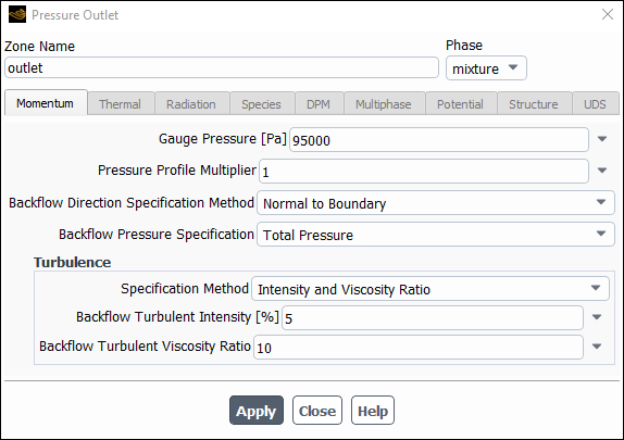
1. Enter 95000 for Gauge Pressure.
2. Retain the default settings in the Turbulence group box.
3. Click Apply and close the Pressure Outlet dialog box.
Set the boundary conditions at outlet for the secondary phase.
Setup → Boundary Conditions → outlet
1. Select vapor from the Phase drop-down list.
2. Click Edit... to open the Pressure Outlet dialog box.
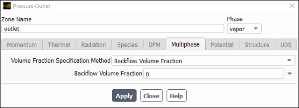
  1. In the Multiphase tab, retain the default value of 0 for Backflow Volume Fraction.
  2. Click Apply and close the Pressure Outlet dialog box.

23.4.8. Operating Conditions

Set the operating pressure.
Setup → Boundary Conditions → Operating Conditions...
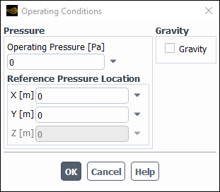
1. Enter 0 Pa for Operating Pressure.
2. Click OK to close the Operating Conditions dialog box.

23.4.9. Solution

Set the solution parameters.
Solution → Solution → Methods...
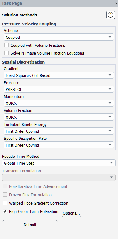
1. Select Coupled from the Scheme drop-down list in the Pressure-Velocity Coupling group box.
2. Retain the selection of PRESTO! from the Pressure drop-down list in the Spatial Discretization group box.
3. Select QUICK for Momentum and Volume Fraction.
4. Retain First Order Upwind for Turbulent Kinetic Energy and Turbulent Dissipation Rate.
5. Select Global Time Step from the Pseudo Time Method drop-down list.
6. Enable High Order Term Relaxation.
  The relaxation of high order terms will help to improve the solution behavior of flow simulations when higher order spatial discretizations are used (higher than first).
Set the solution controls.
Solution → Controls → Controls...
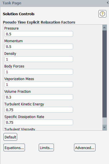
1. Set the pseudo time explicit relaxation factor for Volume Fraction to 0.3.
Enable the plotting of residuals during the calculation.
Solution → Reports → Residuals...
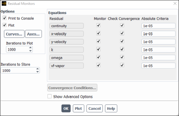
1. Ensure that Plot is enabled in the Options group box.
2. Enter 1e-05 for the Absolute Criteria of continuity, x-velocity, y-velocity, k, omega, and vf-vapor.
  Decreasing the criteria for these residuals will improve the accuracy of the solution.
3. Click OK to close the Residual Monitors dialog box.
Initialize the solution.
Solution → Initialization
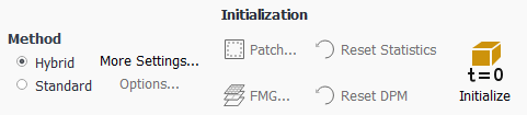
1. Select Hybrid from the Initialization group box.
2. Click More Settings... to open the Hybrid Initialization dialog box.
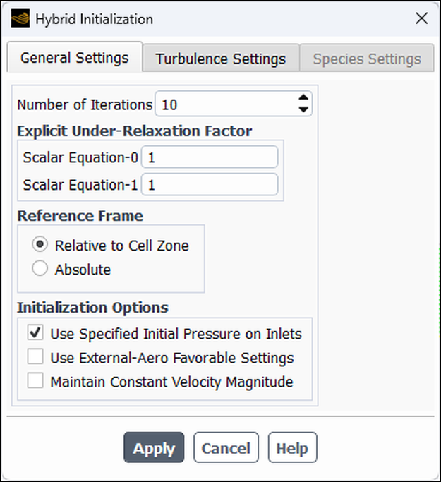
3. Enable Use Specified Initial Pressure on Inlets in the Initialization Options group box. The velocity will now be initialized to the Initial Gauge Pressure value that you set in the Pressure Inlet boundary condition dialog box. For more information on initialization options, see hybrid initialization in the Fluent User's Guide.
4. Click Apply and close the Hybrid Initialization dialog box.
5. Click Initialize to initialize the solution.
  Note: For flows in complex topologies, hybrid initialization will provide better initial velocity and pressure fields than standard initialization. This will help to improve the convergence behavior of the solver.
Save the case file (cav.cas.h5).
File → Write → Case...
Start the calculation by requesting 500 iterations.
Solution → Run Calculation → Run Calculation...
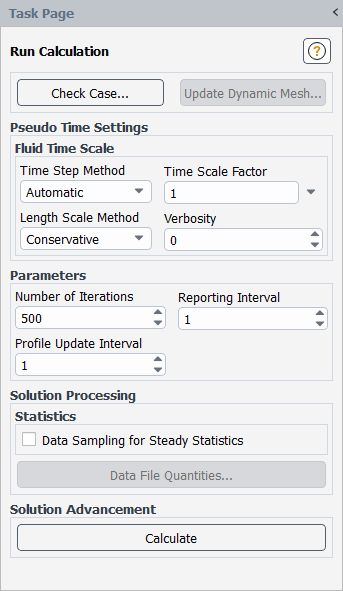
1. Enter 500 for Number of Iterations.
2. Click Calculate.
Save the case and data files (cav.cas.h5 and cav.dat.h5).
File → Write → Case & Data...

23.4.10. Postprocessing

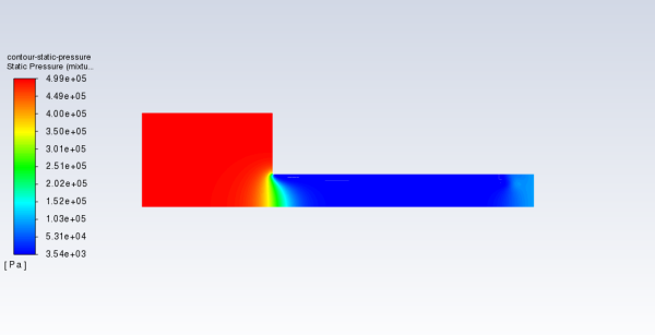
Create and plot a definition of pressure contours in the orifice (Figure 23.3: Contours of Static Pressure).
Results → Graphics → Contours → New...
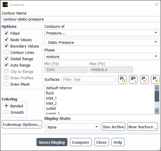
1. Change Contour Name to contour-static-pressure
2. Enable Filled in the Options group box.
3. Enable Banded in the Coloring group box.
4. Retain the default selection of Pressure... and Static Pressure from the Contours of drop-down lists.
5. Click Save/Display and close the Contours dialog box.
  The contour-static-pressure contour definition appears under the Results/Graphics/Contours tree branch. Once you create a plot definition, you can use a right-click menu to display this definition at a later time, for instance, in subsequent simulations with different settings ;or in combination with other plot definitions.
Figure 23.3: Contours of Static Pressure

Note the dramatic pressure drop at the flow restriction in Figure 23.3: Contours of Static Pressure. Low static pressure is the major factor causing cavitation. Additionally, turbulence contributes to cavitation due to the effect of pressure fluctuation (Figure 23.4: Mirrored View of Contours of Static Pressure) and turbulent diffusion (Figure 23.5: Contours of Turbulent Kinetic Energy).
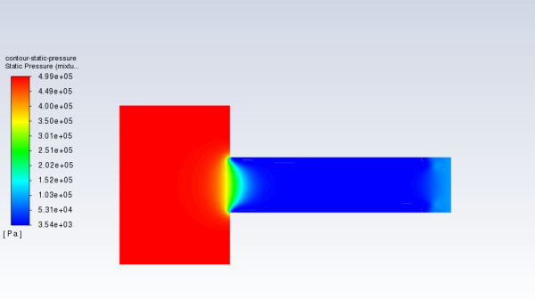
Mirror the display across the centerline (Figure 23.4: Mirrored View of Contours of Static Pressure).
View → Display → Views...
Mirroring the display across the centerline gives a more realistic view.
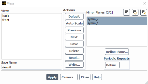
1. Select symm_2 and symm_1 from the Mirror Planes selection list.
2. Click Apply and close the Views dialog box.
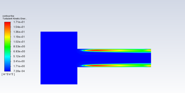
Figure 23.4: Mirrored View of Contours of Static Pressure
Create and plot a contour definition of the turbulent kinetic energy (Figure 23.5: Contours of Turbulent Kinetic Energy).
Results → Graphics → Contours → New...
1. Change Contour Name to contour-tke
2. Enable Filled in the Options group box.
3. Enable Banded in the Coloring group box.
4. Select Turbulence... and Turbulent Kinetic Energy(k) from the Contours of drop-down lists.
5. Click Save/Display.
Figure 23.5: Contours of Turbulent Kinetic Energy

In this example, the mesh used is fairly coarse. However, in cavitating flows the pressure distribution is the dominant factor, and is not very sensitive to mesh size.
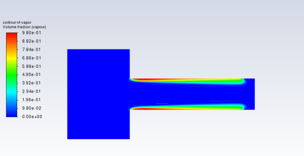
Create and plot a contour definition of the volume fraction of water vapor (Figure 23.6: Contours of Vapor Volume Fraction).
Results → Graphics → Contours → New...
1. Change Contour Name to contour-vf-vapor
2. Enable Filled in the Options group box.
3. Enable Banded in the Coloring group box.
4. Select Phases... and Volume fraction from the Contours of drop-down lists.
5. Select vapor from the Phase drop-down list.
6. Click Save/Display and close the Contours dialog box.
Figure 23.6: Contours of Vapor Volume Fraction

The high turbulent kinetic energy region near the neck of the orifice in Figure 23.5: Contours of Turbulent Kinetic Energy coincides with the highest volume fraction of vapor in Figure 23.6: Contours of Vapor Volume Fraction. This indicates the correct prediction of a localized high phase change rate. The vapor then gets convected downstream by the main flow.
Save the case file (cav.cas.h5).
File → Write → Case...

23.5. Summary

This tutorial demonstrated how to set up and resolve a strongly cavitating pressure-driven flow through an orifice, using multiphase mixture model of Ansys Fluent with cavitation effects. You learned how to set the boundary conditions for an internal flow. A steady-state solution was calculated to simulate the formation of vapor in the neck of the flow after the section restriction at the orifice. A more computationally intensive transient calculation is necessary to accurately simulate the irregular cyclic process of bubble formation, growth, filling by water jet re-entry, and break-off.