Chapter 29: Modeling Two-Way Fluid-Structure Interaction (FSI) Within Fluent

This tutorial is divided into the following sections:

29.1. Introduction

This tutorial examines turbulent air flow through a duct that includes vertical flaps. You will enable a structural model in order to simulate the deformation of the flaps as a result of the fluid flow. It is assumed that the deformation will be large enough that this problem must be modeled as a two-way fluid-structure interaction (FSI) simulation; that is, the fluid flow will affect the deformation of the structures, and vice versa. Because Fluent performs all of the structural calculations (as opposed to using a separate structural program), it is referred to as "intrinsic FSI".

This tutorial demonstrates how to do the following:

Run a journal file to complete an initial steady-state fluid flow simulation without structural calculations.
Set up a transient calculation.
Enable a structural model.
Define structural material properties, a solid cell zone, and related boundary conditions.
Set up dynamic mesh zones for the fluid-structure interaction.
Create solution animation definitions for a scene, contour, and mesh.
Complete a two-way FSI simulation.
Postprocess the fluid flow and the deformation of a solid cell zone.

29.2. Prerequisites

This tutorial is written with the assumption that you have completed the introductory tutorials found in this manual and that you are familiar with the Ansys Fluent outline view and ribbon structure. Some steps in the setup and solution procedure will not be shown explicitly.

29.3. Problem Description

The problem to be modeled in this tutorial is shown schematically in Figure 29.1: Problem Schematic.

Figure 29.1: Problem Schematic

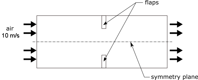
Flow through a simple duct with vertical flaps is simulated as a 2D planar model. The duct is 10 cm long and 4 cm high, and the flaps are 1 cm tall and 0.3 cm thick, composed of silicone rubber. Turbulent air enters the duct at 10 m/s, flows around the flaps, and exits through a pressure outlet. Symmetry allows only half of the duct to be modeled.

29.4. Setup and Solution

The following sections describe the setup and solution steps for this tutorial:

29.4.1. Preparation

To prepare for running this tutorial:

Download the fsi_2way.zip file here .
Unzip fsi_2way.zip to your working directory.
The files flap.msh and steady_fluid_flow.jou can be found in the folder. Note that the cell zone in the mesh file that will represent the solid zone is appropriate for a 2D intrinsic FSI simulation, which requires that only quadrilateral and/or triangular cell types are used and that a conformal mesh exists between the zones that will represent the solid and the fluid.
Use the Fluent Launcher to start Ansys Fluent.
Select Solution in the top-left selection list to start Fluent in Solution Mode.
Select 2D under Dimension.
Enable Double Precision under Options.
Retain the default Solver Processes to 1 under Parallel (Local Machine).
Make sure that the Working Directory (in the General Options tab) is set to the one created when you unzipped fsi_2way.zip.
Read the journal file steady_fluid_flow.jou.
File → Read → Journal...
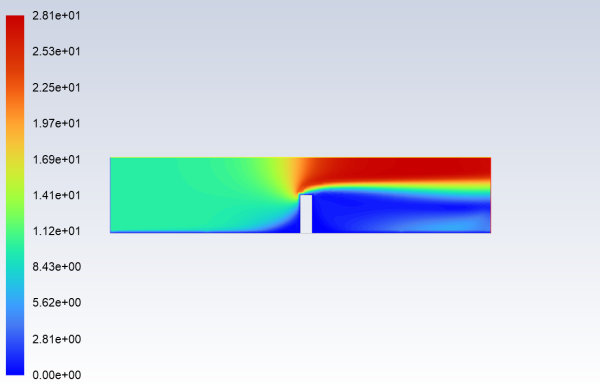
This journal file will read the mesh file flap.msh and set up and solve a steady fluid flow simulation that will serve as the starting point for the transient FSI simulation. Solving the steady flow problem first allows you to easily discern and resolve any convergence issues that are not related to the fluid-structure interaction.
As Fluent reads the journal file, it will report the text commands and solution progress in the console. You can also view the journal file in a text editor to see the settings used in this simulation. The final text command in the journal file will display contours of the velocity magnitude (Figure 29.2: Steady-State Velocity Magnitude).
Figure 29.2: Steady-State Velocity Magnitude
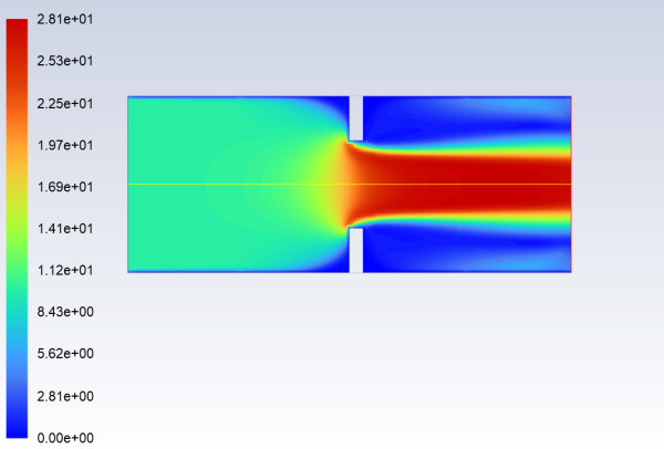
Mirror the display across the centerline (Figure 29.3: Duct with Mirroring).
View → Display → Views...
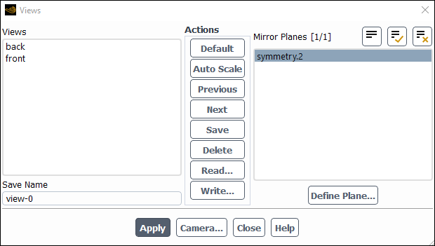
1. Select symmetry.2 in the Mirror Planes selection list.
2. Click Apply to refresh the display.
3. Close the Views dialog box and reposition the view as shown in Figure 29.3: Duct with Mirroring.
Figure 29.3: Duct with Mirroring
Save the initial case and data files as flap_fluid.cas.h5 and flap_fluid.dat.h5.
File → Write → Case & Data...

Having completed an initial steady fluid flow simulation, the remaining steps are all concerned with setting up the structural calculations and obtaining the transient results for the deformation of the solid flaps.

29.4.2. Solver and Analysis Type

Specify the solver settings.
Setup → General
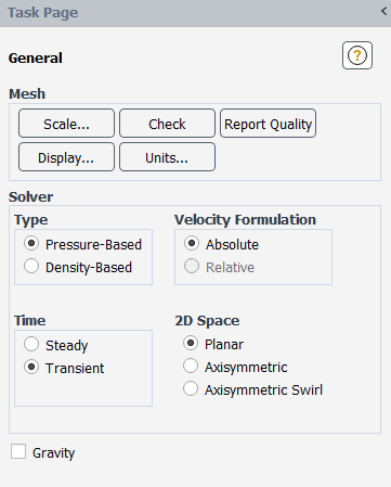
1. Enable a time-dependent calculation by selecting Transient in the General task page (Solver group).
2. Retain the default selection of Pressure-Based from the Type list.

29.4.3. Structural Model

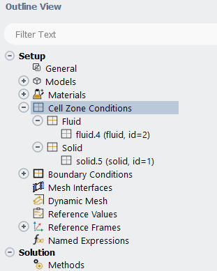
Verify that a solid cell zone is already defined, as this is necessary to be able to enable a structural model. You can view the existing cell zones in the Outline View window.
Enable the linear elasticity structural model.
Setup → Models → Structure Edit...
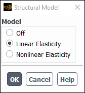
1. Select Linear Elasticity from the Model list.
  This model enables structural calculations for the solid cell zone such that the internal load is linearly proportional to the nodal displacement, and the structural stiffness matrix remains constant.
2. Click OK to close the Structural Model dialog box.

29.4.4. Materials

Create a new solid material for the flap.
Setup → Materials → Solid New...
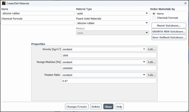
1. Enter silicone-rubber for the Name.
2. Clear the Chemical Formula field.
3. Enter 1600 for the Density.
4. Enter 1e+6 for the Youngs Modulus.
5. Enter 0.47 for the Poisson Ratio.
6. Click Change/Create, and click Yes in the Question dialog box to overwrite aluminum.
7. Close the Create/Edit Materials dialog box.

29.4.5. Cell Zone Conditions

Set up the cell zone conditions for the solid zone associated with the flap (solid.5).
Setup → Cell Zone Conditions → Solid → solid.5 Edit...
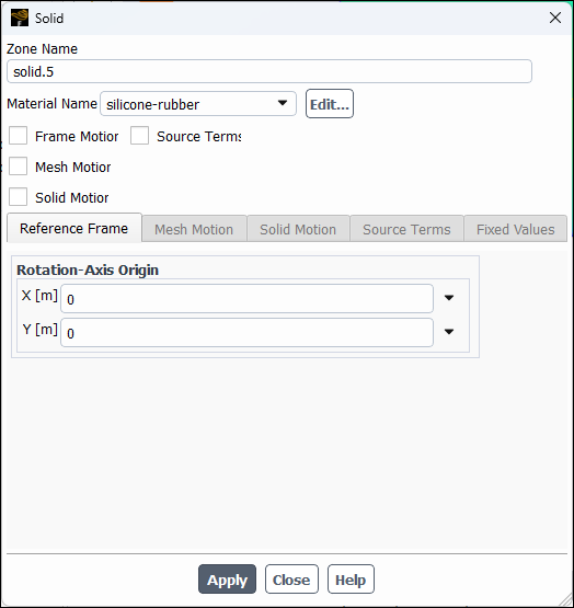
1. Select silicone-rubber from the Material Name drop-down list.
2. Click Apply and close the Solid dialog box.

29.4.6. Boundary Conditions

You must ensure that the boundary conditions are appropriately defined for every wall that is immediately adjacent to the solid zone.

Set the boundary conditions for flap_attach, which is located where the flap attaches to the duct. You will define it as being fixed (that is, undergoing no displacement).
Setup → Boundary Conditions → Wall → flap_attach Edit...
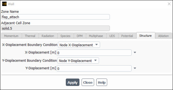
1. In the Structure tab, select displacement boundary conditions (that is, Node X-Displacement from the X-Displacement Boundary Condition drop-down list with 0 for the X-Displacement, and so on).
2. Click Apply and close the Wall dialog box.
Set the boundary conditions for all of the two-sided walls (that is, the wall / wall-shadow pairs) between the solid and fluid cell zones. In this case there is one pair of walls, which represent the outer surface of the flap.
1. Set the boundary conditions for flap_wall-shadow.
  Setup → Boundary Conditions → Wall → flap_wall-shadow Edit...
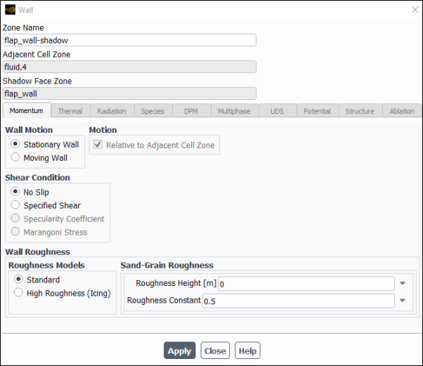
  Note that the Adjacent Cell Zone for this wall is fluid.4, which is the fluid zone. The side of the wall / wall-shadow pair that is immediately adjacent to the fluid does not require any settings in the Structure tab, and so this tab is not available.
  1. Retain the default settings in the Momentum tab.
  2. Click Apply and close the Wall dialog box.
2. Set the boundary conditions for flap_wall.
  Setup → Boundary Conditions → Wall → flap_wall Edit...
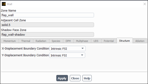
  Note that the Adjacent Cell Zone for this wall is solid.5, which is the solid zone. The side of the wall / wall-shadow pair that is immediately adjacent to the solid does require structural settings (that is, displacement boundary conditions).
  1. Click the Structure tab.
  2. Select Intrinsic FSI from the X- and Y-Displacement Boundary Condition drop-down lists.
    This specifies that the displacement results from pressure loads exerted by the fluid flow on the faces. This setting is only available for two-sided walls.
  3. Click Apply and close the Wall dialog box.

29.4.7. Dynamic Mesh Zones

For two-way FSI simulations, you must define dynamic mesh properties to allow the mesh to handle the deformation of the solid zone.

Domain → Mesh Models → Dynamic Mesh...

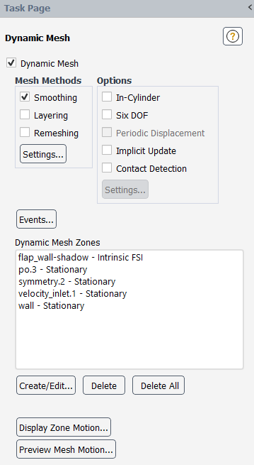
Enable the Dynamic Mesh option.
Make sure that the Smoothing option is enabled in the Mesh Methods group box, and click the Settings... button to open the Mesh Method Settings dialog box.
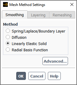
1. Select Linearly Elastic Solid from the Method list.
2. Click OK to close the Mesh Method Settings dialog box.
Retain the default settings in the Options group box (that is, with the options disabled). These options are not supported for FSI simulations, except for Implicit Update. The Implicit Update option may be required for more complex cases in which the stability of the FSI simulation may be an issue, but for a simple case such as this one, it is not required.
Click the Create/Edit... button to open the Dynamic Mesh Zones dialog box.
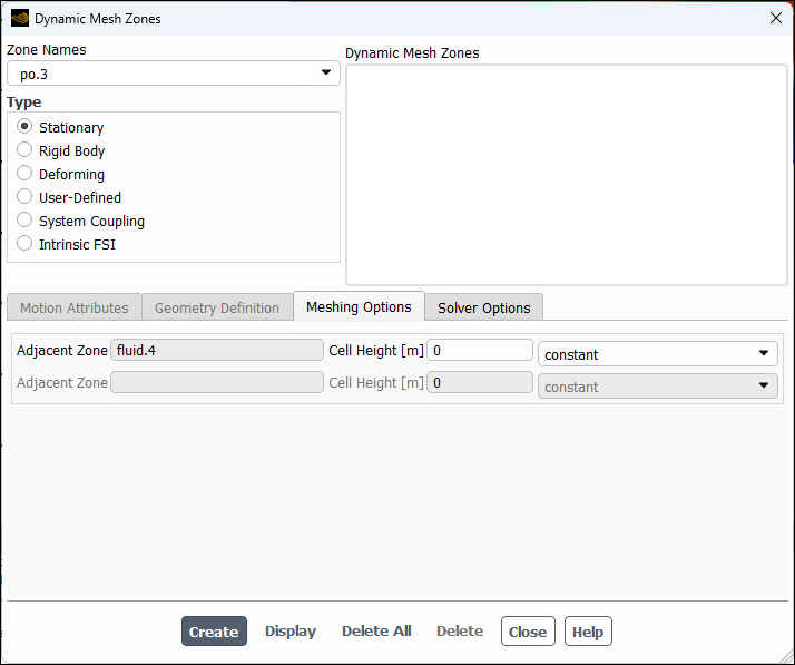
1. Select po.3 (the pressure outlet) from the Zone Names drop-down list, select Stationary from the Type list, and click Create. This ensures the boundary zone does not deform.
2. In a similar manner, create stationary dynamic zones for the other boundary zones that are not deforming: symmetry.2, velocity_inlet.1, and wall.
3. Select flap_wall-shadow (the side of the wall / wall-shadow pair that is immediately adjacent to the fluid) from the Zone Names drop-down list, select Intrinsic FSI from the Type list, and click Create. This specifies that the wall / wall-shadow pair deforms according to the deformation of the adjacent solid zone.
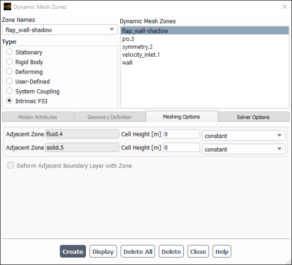
4. Close the Dynamic Mesh Zones dialog box.

29.4.8. Solution Animations

By setting up animation definitions, you will be able to capture results for your transient simulation as it calculates the solution, so that you can later display how the fluid flow and flap shape change over time.

Create a scene that can be used in an animation definition for the fluid flow.
Scenes are used when you want to display multiple graphics objects within a single window. In this case, the animation will include not only contours of the fluid velocity, but also boundary zones.
Results → Scene New...
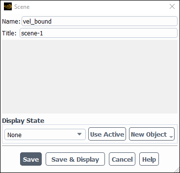
1. Enter vel_bound for the Name.
2. Click New Object and select Mesh... from the drop-down list to open the associated dialog box.
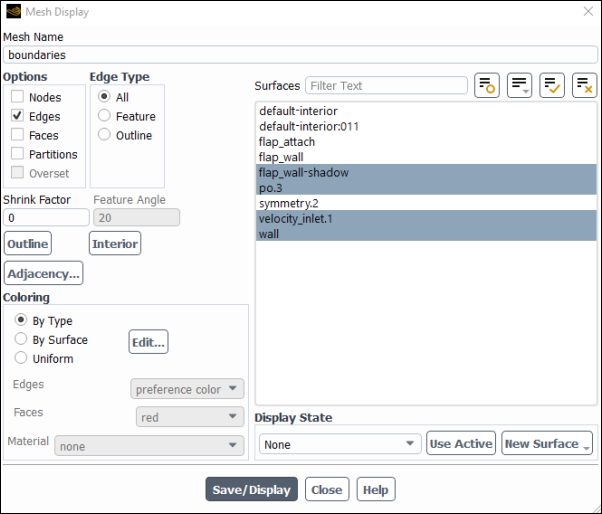
  1. Enter boundaries for the Mesh Name.
  2. Select Edges under the Options list.
  3. Deselect all surfaces in the Surfaces selection list by clicking , and then select flap_wall-shadow, po.3, velocity_inlet.1, and wall.
  4. Click Save/Display and close the Mesh Display dialog box.
3. Click New Object and select Contours... from the drop-down list to open the associated dialog box.
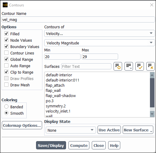
  1. Enter vel_mag for the Contour Name.
  2. Select Velocity... and Velocity Magnitude from the Contours of drop-down lists.
  3. Disable the Auto Range option and enter 20 and 29 for the Min and Max, respectively.
    Disabling the Auto Range ensures that all of the results in the animation have the same scale. The velocity of the fluid will not change very much in this particular solution, and so using a narrow range of values will make it easier to identify the small contour changes.
  4. Deselect all surfaces in the Surfaces selection list by clicking .
    For 2D cases, if no surface is selected, contouring is done on the entire domain.
  5. Click the Save/Display button and close the Contours dialog box.
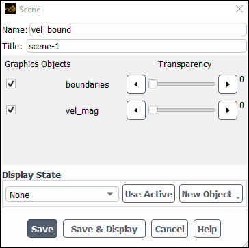
4. Click the Save & Display button, and then click Cancel to close the Scene dialog box.
Create an animation definition for the fluid velocity and boundaries scene.
Solution → Calculation Activities → Solution Animations New...
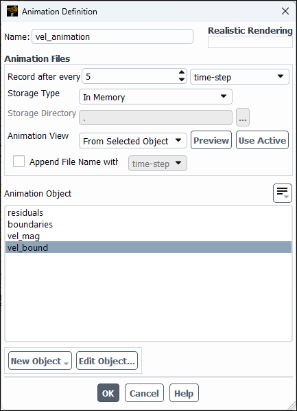
1. Enter vel_animation for the Name.
2. Enter 5 for Record after every and select iteration from the drop-down list.
3. Select In Memory from the Storage Type drop-down.
  The In Memory option is acceptable for a small 2D case such as this. For larger 2D or 3D cases, saving animation files with either the PPM Image or HSF File option is preferable, to avoid using too much of your machine’s memory.
4. Select vel_bound from the Animation Object list.
5. Click OK to create the animation definition.
Create an animation definition for the flap displacement.
Solution → Calculation Activities → Solution Animations New...
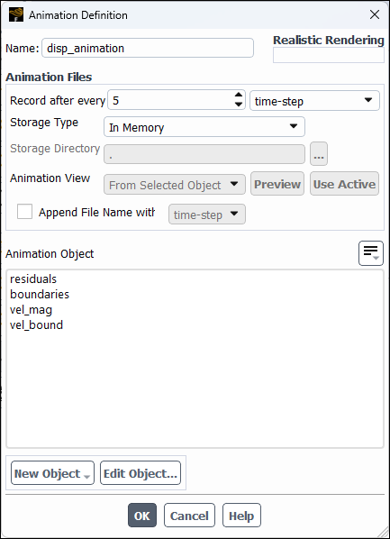
1. Enter disp_animation for the Name.
2. Enter 5 for Record after every and select iteration from the drop-down list.
3. Select In Memory from the Storage Type drop-down.
4. Click New Object and select Contours... from the drop-down list to open the associated dialog box.
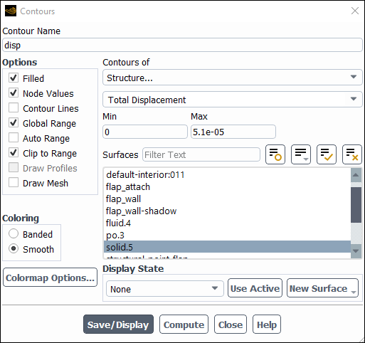
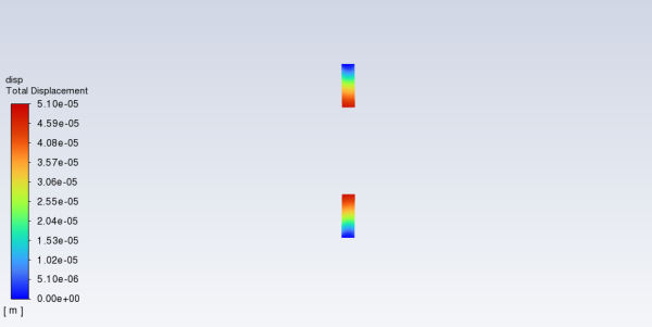
  1. Enter disp for the Contour Name.
  2. Select Structure... and Total Displacement from the Contours of drop-down lists.
  3. Disable Auto Range and enter 0 and 5.1e-05 for Min and Max, respectively.
  4. Select solid.5 from the Surfaces list.
  5. Click Save/Display and close the Contours dialog box.
5. Select disp from the Animation Object list.
6. Click OK to create the animation definition.
Create an animation definition for the mesh.
Solution → Calculation Activities → Solution Animations New...
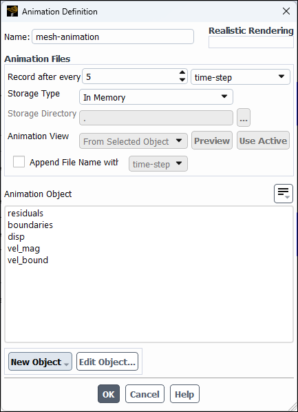
1. Enter mesh_animation for the Name.
2. Enter 5 for Record after every and select iteration from the drop-down list.
3. Select In Memory from the Storage Type drop-down.
4. Click New Object and select Mesh... from the drop-down list to open the associated dialog box.
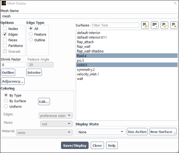
  1. Enter mesh for the Mesh Name.
  2. Disable the Faces option.
  3. Deselect all surfaces in the Surfaces selection list by clicking , and then select fluid.4 and solid.5.
  4. Click Save/Display and close the Mesh Display dialog box.
5. Select mesh from the Animation Object list.
6. Click OK to create the animation definition.
Add a structural point surface to a location of interest within the solid zone.
Results → Surfaces New → Structural Point...
The Structural Point Surface dialog appears, as does a point triad in the graphics window. Zoom into the mesh displayed in the graphics window to focus on the tip of the flap.
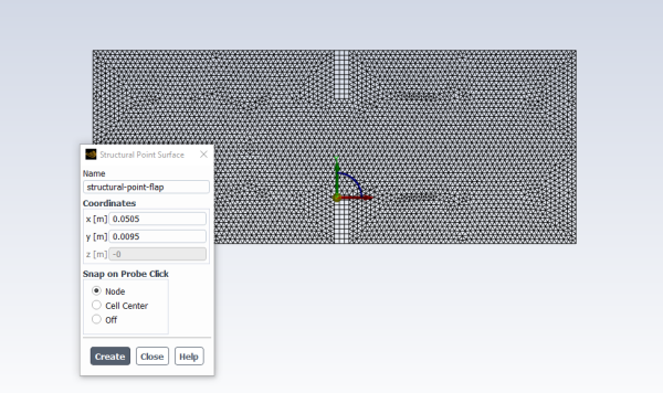
1. Enter structural-point-flap for the Name.
2. Enter 0.0505 for the x coordinate, and enter 0.0095 for the y coordinate.
  Alternatively,you can use the mouse to drag the point's position in the graphics window to an approximate location.
3. Click Create to create the structural point surface at this location.
4. Close the Structural Point Surface dialog box.
Create a report definition to monitor displacement of the flap.
Solution → Report Definitions New → Surface Report → Vertex Average...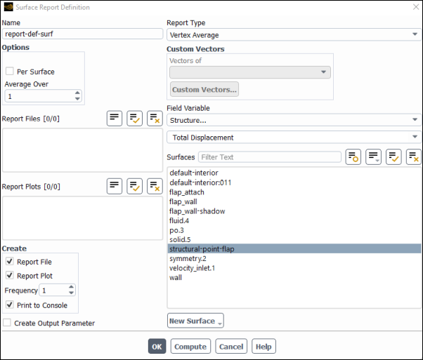
1. Enter report-def-surf for the Name.
2. Select Structure... and Total Displacement from the Contours of drop-down lists.
3. Select structural-point-flap from the Surfaces list.
4. Enable the Report File, Report Plot, and Print to Console options.
5. Click OK.
This report definition will monitor and plot the vertex average of the displacement of the nodes that surround the structural point surface.

29.4.9. Solution

Disable the checking of convergence for the displacement residual equations.
Solution → Monitors → Residual Edit...
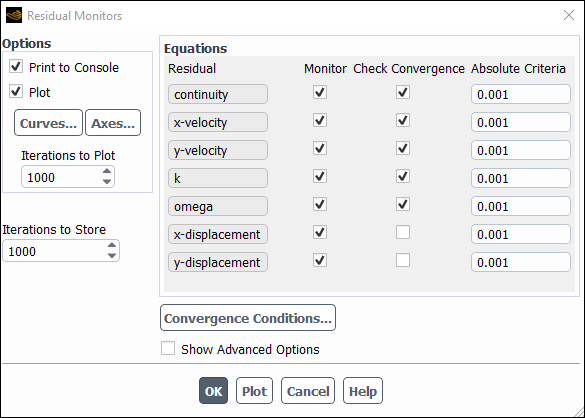
1. Disable the Check Convergence options for the x- and y-displacement equations.
2. Click OK to close the Residual Monitors dialog box.
Save the case file (flap_fsi_2way.cas.h5).
File → Write → Case...
Start the calculation.
Solution → Run Calculation → 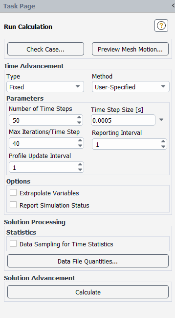Run Calculation...
1. Enter 50 for Number of Time Steps.
2. Enter 0.0005 for Time Step Size.
3. Enter 40 for Max Iterations/Time Step.
4. Click Calculate.
After the solution has been calculated, save the case and data files (flap_fsi_2way.cas.h5 and flap_fsi_2way.dat.h5).
File → Write → Case & Data...

29.4.10. Postprocessing

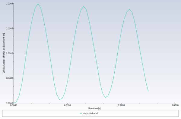
View the displacement of the flap's point surface (Figure 29.4: The Vertex Average Displacement of the Flap's Point Surface).
Figure 29.4: The Vertex Average Displacement of the Flap's Point Surface

The monitored plot of the vertex average of the displacement at the point surface clearly shows displacement over time.
View the animations of the results.
Results → Animations → Playback Edit...
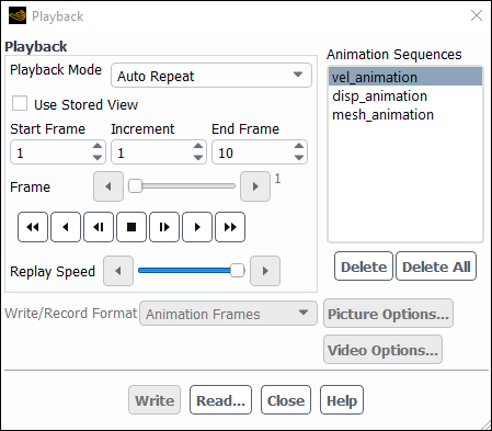
1. Select Auto Repeat from the Playback Mode drop-down list.
2. Disable the Use Stored View option.
3. Select vel_animation from the Animation Sequences list.
4. Decrease the Replay Speed by clicking the button four times.
5. Click the play button (the second from the right in the group of buttons in the Playback group box).
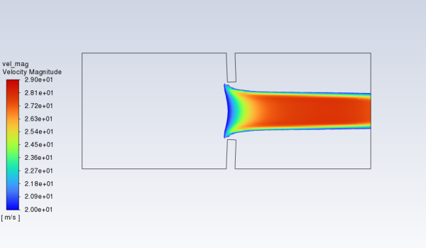
6. Magnify the view as shown in Figure 29.5: Contours of Velocity Magnitude.
  Figure 29.5: Contours of Velocity Magnitude
7. Click the button to stop the animation.
8. Select disp_animation from the Animation Sequences list.
9. Click the play button.
10. Magnify the view as shown in Figure 29.6: Contours of Total Displacement.
  Figure 29.6: Contours of Total Displacement
11. Click the button to stop the animation.
12. Select mesh_animation from the Animation Sequences list.
13. Click the play button.
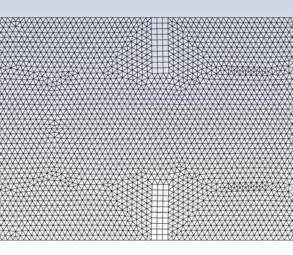
14. Magnify the view as shown in Figure 29.7: The Mesh of the Displaced Flap.
  Figure 29.7: The Mesh of the Displaced Flap
15. Click the button to stop the animation.

29.5. Summary

This tutorial demonstrated how to set up and solve a two-way intrinsic FSI simulation. You learned how to enable a structural model and define the solid material, boundary conditions, and dynamic mesh zones. After completing the simulation, you viewed animations of the resulting fluid velocity contours and displacement of the structure. For more information about intrinsic FSI simulations, see the Fluent User's Guide.