Chapter 28: Modeling One-Way Fluid-Structure Interaction (FSI) Within Fluent

This tutorial is divided into the following sections:

28.1. Introduction

This tutorial examines turbulent air flow through a cylindrical test chamber that includes a steel probe. You will enable a structural model in order to simulate the deformation of the probe as a result of the fluid flow. It is assumed that the deformation will be small enough that this problem can be modeled as a one-way fluid-structure interaction (FSI) simulation; that is, the fluid flow will affect the deformation of the structure, but not vice versa. Because Fluent performs all of the structural calculations (as opposed to using a separate structural program), it is referred to as "intrinsic FSI".

This tutorial demonstrates how to do the following:

Run a journal file to complete an initial fluid flow simulation without structural calculations.
Enable a structural model.
Define structural material properties, a solid cell zone, and related boundary conditions.
Turn off flow and turbulence equations.
Complete a one-way FSI simulation.
Postprocess the deformation of a solid cell zone.

28.2. Prerequisites

This tutorial is written with the assumption that you have completed the introductory tutorials found in this manual and that you are familiar with the Ansys Fluent outline view and ribbon structure. Some steps in the setup and solution procedure will not be shown explicitly.

28.3. Problem Description

The problem to be modeled in this tutorial is shown schematically in Figure 28.1: Problem Schematic.

Figure 28.1: Problem Schematic

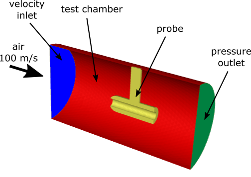
Taking advantage of the symmetry of the problem, only half of the geometry is modeled. The cylindrical test chamber is 20 cm long, with a diameter of 10 cm. Turbulent air enters the chamber at 100 m/s, flows around and through the steel probe, and exits through a pressure outlet.

28.4. Setup and Solution

The following sections describe the setup and solution steps for this tutorial:

28.4.1. Preparation

To prepare for running this tutorial:

Download the fsi_1way.zip file here .
Unzip fsi_1way.zip to your working directory.
The files probe.msh.h5 and fluid_flow.jou can be found in the folder. Note that the solid cell zone in the mesh file is appropriate for a 3D intrinsic FSI simulation, which requires that only hexahedral, tetrahedral, wedge, and/or pyramid cell types are used and that a conformal mesh exists between the solid and fluid zones.
Use the Fluent Launcher to start Ansys Fluent.
Select Solution in the top-left selection list to start Fluent in Solution Mode.
Select 3D under Dimension.
Enable Double Precision under Options.
Retain the default Solver Processes to 1 under Parallel (Local Machine).
Make sure that the Working Directory (in the General Options tab) is set to the one created when you unzipped fsi_1way.zip.
Read the journal file fluid_flow.jou.
File → Read → Journal...
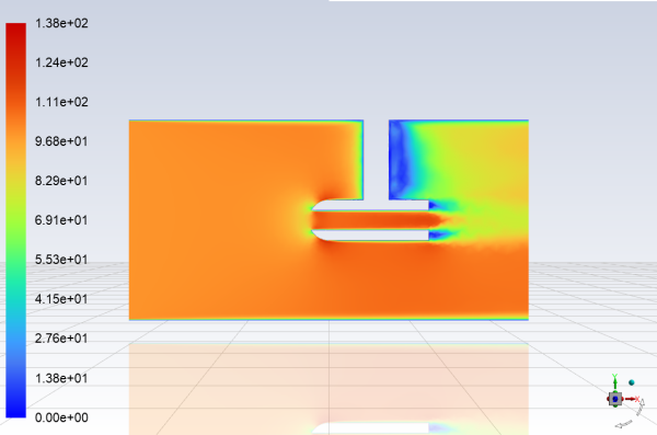
This journal file will read the mesh file probe.msh.h5 and set up and solve a fluid flow simulation that will serve as the starting point for the structural calculations. It is not necessary to separate these calculations, but it is a advantage of one-way FSI simulation that structural calculations can be simply added to an existing fluid flow case and data file. Separating the calculations allows you to easily discern and resolve any convergence issues that are solely related to the fluid simulation.
As Fluent reads the journal file, it will report the text commands and solution progress in the console. You can also view the journal file in a text editor to see the settings used in this simulation. The final text command in the journal file will display contours of the velocity magnitude (Figure 28.2: Velocity Magnitude on the Symmetry Plane).
Figure 28.2: Velocity Magnitude on the Symmetry Plane
Save the initial case and data files as probe_fluid.cas.h5 and probe_fluid.dat.h5.
File → Write → Case & Data...

Having completed the initial fluid flow simulation, the remaining steps are all concerned with setting up the structural calculations and obtaining the deformation results for the solid cell zone as a result of the flow pressure.

28.4.2. Structural Model

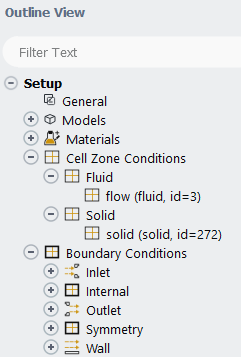
Verify that a solid cell zone is already defined, as this is necessary to be able to enable a structural model. You can view the existing cell zones in the Outline View window.
Enable the linear elasticity structural model.
Setup → Models → Structure Edit...
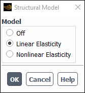
1. Select Linear Elasticity from the Model list.
  This model enables structural calculations for the solid cell zone such that the internal load is linearly proportional to the nodal displacement, and the structural stiffness matrix remains constant.
2. Click OK to close the Structural Model dialog box.

28.4.3. Materials

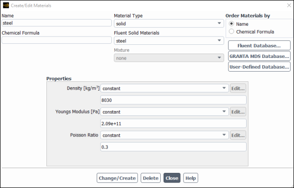
Add steel to the list of solid materials by copying it from the Ansys Fluent materials database.
Setup → Materials → Solid → aluminum Edit...
1. Click the Fluent Database... button in the Create/Edit Materials dialog box to open the Fluent Database Materials dialog box.
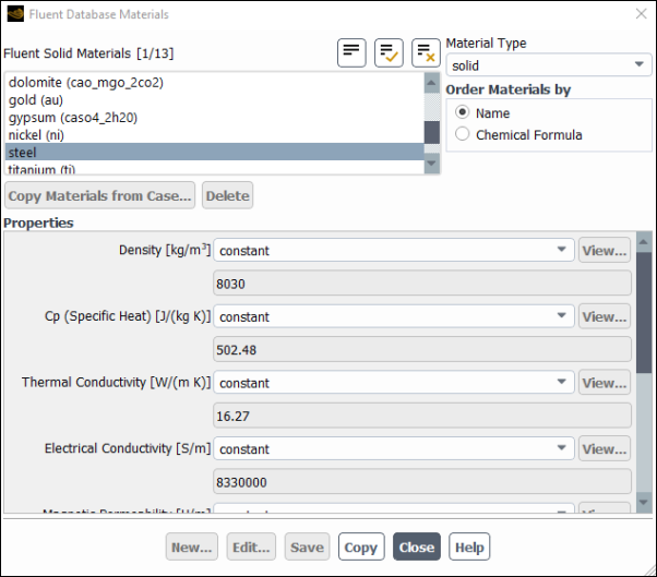
2. Select solid from the Material Type drop-down list.
3. Select steel in the Fluent Solid Materials selection list.
  Scroll down the list to find steel. Selecting this item will display the default properties in the dialog box.
4. Click Copy, then close the Fluent Database Materials dialog box.
  The Create/Edit Materials dialog box will now display the copied properties for steel.
5. Keep the default values for the material.
6. Click Change/Create and close the Create/Edit Materials dialog box.

28.4.4. Cell Zone Conditions

Set up the cell zone conditions for the solid zone associated with the probe (solid).
Setup → Cell Zone Conditions → Solid → solid Edit...
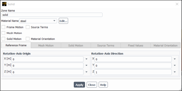
1. Select steel from the Material Name drop-down list.
2. Click Apply and close the Solid dialog box.

28.4.5. Boundary Conditions

You must ensure that the boundary conditions are appropriately defined for every wall that is immediately adjacent to the solid zone.

Set the boundary conditions for solid-top, which is located where the probe attaches to the top of the test chamber. You will define it as being fixed (that is, undergoing no displacement).
Setup → Boundary Conditions → Wall → solid-top Edit...
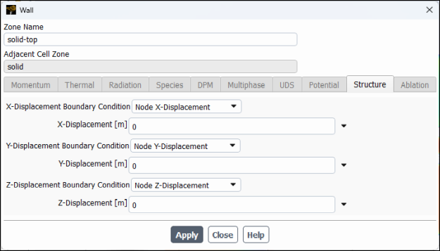
1. Click the Structure tab.
2. Select displacement boundary conditions (that is, Node X-Displacement from the X-Displacement Boundary Condition drop-down list with 0 for the X-Displacement, and so on).
3. Click Apply and close the Wall dialog box.
Set the boundary conditions for all of the wall zones of the solid cell zone that lie on the plane of symmetry and represent the center of the probe. In this case there are two: they should be free to move with no stress in the X- and Y-directions, but fixed in the Z-direction.
1. Set the boundary conditions for solid-symmetry.
  Setup → Boundary Conditions → Wall → solid-symmetry Edit...
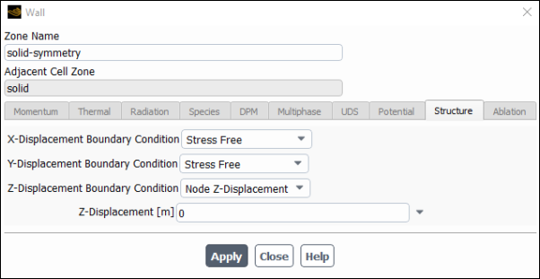
  1. Click the Structure tab.
  2. Select Stress Free from the X- and Y-Displacement Boundary Condition drop-down lists.
  3. Select the Z-Displacement Boundary Condition drop-down list and the Z-Displacement field (that is, Node Z-Displacement and set 0, respectively).
    This ensures that the zone does not move out of the plane of symmetry.
  4. Click Apply and close the Wall dialog box.
2. Copy the boundary conditions from solid-symmetry to solid-symmetry:011.
  Setup → Boundary Conditions → Wall → solid-symmetry Copy...
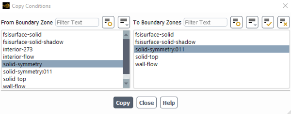
  1. Make sure that solid-symmetry is selected in the From Boundary Zone list.
  2. Select solid-symmetry:011 in the To Boundary Zones list.
  3. Click the Copy button.
    A Question dialog box will open, asking if you want to copy the boundary conditions to all of the selected zones. Click OK.
  4. Close the Copy Conditions dialog box.
Set the boundary conditions for all of the two-sided walls (that is, the wall / wall-shadow pairs) between the solid and fluid cell zones. In this case there is one pair of walls, which represent the outer surface of the probe.
1. Set the boundary conditions for fsisurface-solid-shadow.
  Setup → Boundary Conditions → Wall → fsisurface-solid-shadow Edit...
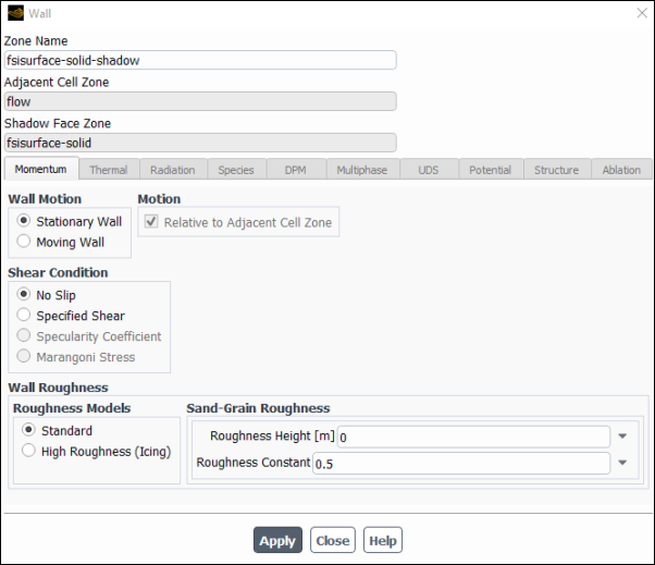
  Note that the Adjacent Cell Zone for this wall is flow, which is the fluid zone. The side of the wall / wall-shadow pair that is immediately adjacent to the fluid does not require any settings in the Structure tab, and so this tab is not available.
  1. Retain the default settings in the Momentum tab.
  2. Click Apply and close the Wall dialog box.
2. Set the boundary conditions for fsisurface-solid.
  Setup → Boundary Conditions → Wall → fsisurface-solid Edit...
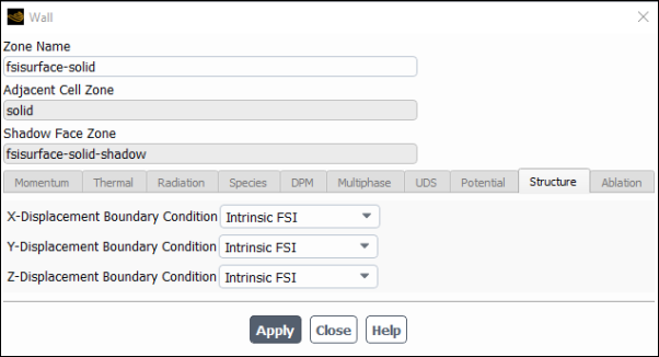
  Note that the Adjacent Cell Zone for this wall is solid, which is the solid zone. The side of the wall / wall-shadow pair that is immediately adjacent to the solid does require structural settings (that is, displacement boundary conditions).
  1. Click the Structure tab.
  2. Select Intrinsic FSI from the X-, Y-, and Z-Displacement Boundary Condition drop-down lists.
    This specifies that the displacement results from pressure loads exerted by the fluid flow on the faces. This setting is only available for two-sided walls.
  3. Click Apply and close the Wall dialog box.

28.4.6. Solution

Enable the inclusion of operating pressure into the fluid-structure interaction force by entering the following text command:
```
> define/models/structure/expert/include-pop-in-fsi-force?
Include operating p into fsi force [no] yes
```
Disable the flow and turbulence equations, since in a one-way FSI simulation they will not change from their converged state.
Solution → Controls Equations...
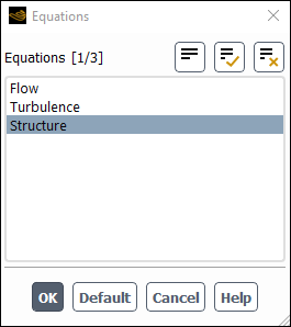
1. Deselect Flow and Turbulence from the Equations selection list.
2. Retain the selection of Structure.
3. Click OK to close the Equations dialog box.
Review the convergence criteria for the displacement residual equations.
Solution → Monitors → Residual Edit...
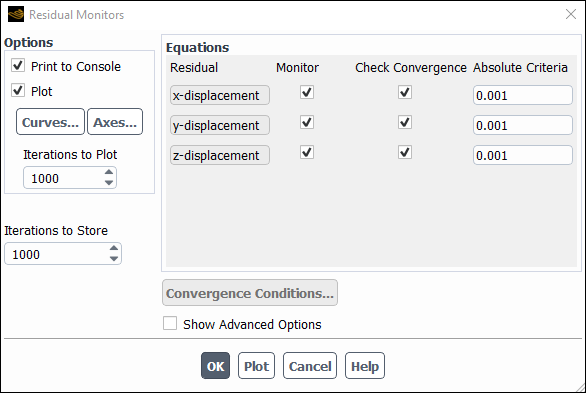
1. Retain the default settings for the x-, y-, and z-displacement equations.
2. Click OK to close the Residual Monitors dialog box.
Save the case file (probe_fsi_1way.cas.h5).
File → Write → Case...
Start the calculation by requesting 2 iterations in the Solution ribbon tab (Run Calculation group box)..
Solution → Run Calculation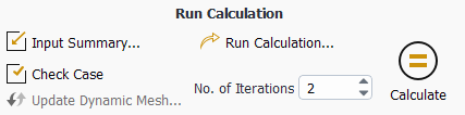
1. Enter 2 for No. of Iterations.
  Since only structural calculations will be performed, you do not need a large number of iterations to reach convergence.
2. Click Calculate.
After the solution has been calculated, save the case and data files (probe_fsi_1way.cas.h5 and probe_fsi_1way.dat.h5).
File → Write → Case & Data...

28.4.7. Postprocessing

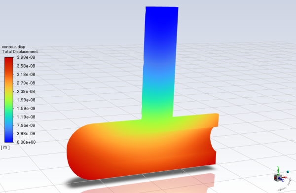
Display the total displacement of the probe (Figure 28.3: Contours of Total Displacement).
Results → Graphics → Contours → New...
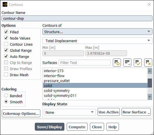
1. Enter contour-disp for Contour Name.
2. Select Structure... and Total Displacement from the Contours of drop-down lists.
3. Deselect all surfaces in the Surfaces selection list by clicking , and then select solid.
4. Click Save/Display, close the Contours dialog box, and rotate and magnify the view as shown in Figure 28.3: Contours of Total Displacement.
  Figure 28.3: Contours of Total Displacement
Save the case file (probe_fsi_1way.cas.h5).
File → Write → Case...

28.5. Summary

This tutorial demonstrated how to set up and solve a one-way intrinsic FSI simulation. You learned how to enable a structural model and define the solid material and boundary conditions. After completing the simulation, you displayed the resulting displacement of the structure. For more information about intrinsic FSI simulations, see the Fluent User's Guide.