


This tutorial is divided into the following sections:
Ansys Fluent’s adjoint solver is used to compute the sensitivity of quantities of interest in a fluid system with respect to the user-specified inputs, for an existing flow solution. Importantly, this also includes the sensitivity of the computed results with respect to the geometric shape of the system. The adjoint design change tool is a powerful component that can use the sensitivity information from one or more adjoint solutions to guide systematic changes that result in predictable improvements in the system performance, which can be made subject to various types of design constraints if desired.
This tutorial provides an example of how to generate sensitivity data for flow past a circular cylinder, how to postprocess the results, and how to use the data to perform a multi-objective design change that reduces drag and increases lift by morphing the mesh. The tutorial makes use of a previously computed flow solution, and demonstrates how to do the following:
Select the observable of interest.
Access the solver controls for advancing the adjoint solution.
Set convergence criteria and plot and print residuals.
Advance the adjoint solver.
Postprocess the results to extract sensitivity data.
Use the design change tool to modify the cylinder shape to simultaneously reduce the drag and increase the lift.
The configuration is a circular cylinder, bounded above and below by symmetry planes. The flow is laminar and incompressible with a Reynolds number of 40, based on the cylinder diameter. At this Reynolds number, the flow is steady.
The following sections describe the setup steps for this tutorial:
Download the
adjoint_cylinder.zipfile here .Unzip
adjoint_cylinder.zipto your working directory.The files
cylinder_tutorial.casandcylinder_tutorial.datcan be found in the folder .Use the Fluent Launcher to start Ansys Fluent.
Select Solution in the top-left selection list to start Fluent in Solution Mode.
Select 2D under Dimension.
Enable Double Precision under Options.
Enable Display Mesh After Reading in the General Options tab.
Load the converged case and data file for the cylinder geometry.
 File → Read →
Case & Data...
File → Read →
Case & Data...
When prompted, browse to the location of the case and data files and select
cylinder_tutorial.casto load. The corresponding data file will automatically be loaded as well.Note: After you read in the mesh, it will be displayed in the embedded graphics windows, since you enabled the appropriate display option in Fluent Launcher.
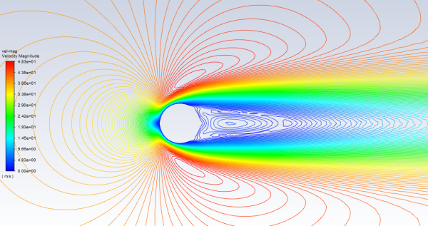
The data file contains a previously computed flow solution that will serve as the starting point for the adjoint calculation. Part of the mesh and the velocity field are shown below:

Begin setting up the adjoint solver by opening the Adjoint Observables dialog box. Here you will create lift and drag observables. Clicking on any button in the Gradient-Based group of the Design ribbon tab will activate the adjoint solver.
![]() Design → Gradient-Based
→ Observable...
Design → Gradient-Based
→ Observable...
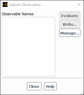
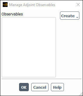
Click the button to open the Manage Adjoint Observables dialog box.
Click the button and select force from the Observable types drop-down list.
The Manage Adjoint Observables will update to show the newly created force-01 observable which must now be configured:
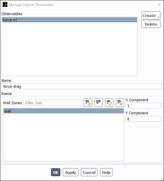
Ensure that force-01 is selected from the Observables list.
Enter
force-dragfor Name.Select wall under Wall Zones. This is the cylinder wall on which you want the force to be evaluated.
Ensure that the X-Component direction is set to
1and the Y-Component direction is set to0.Click to commit the settings for force-drag. Upon clicking , force-01 will be renamed to force-drag.
Repeat the process in the Manage Adjoint Observables dialog box to create a lift observable with the following settings:
Name force-liftWall Zones wallX-Component 0Y-Component 1When you have configured the force-lift observable, click to commit the settings for force-lift and close the Manage Adjoint Observables dialog box.
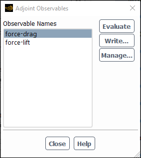
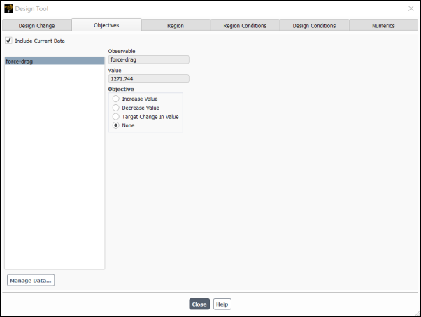
In the Adjoint Observables dialog box (Figure 30.5: Adjoint Observables Dialog Box) specify that you will solve for the drag sensitivity.
Select in the list of Observable Names.
The selection in the Adjoint Observables dialog box determines the observable for which sensitivities will be computed. You will first compute the drag sensitivities.
Click to print the value of the drag force on the wall in the console.
Observable name: force-drag
Observable Value [N] = 1271.7444
This value is in SI units, with
Ndenoting Newtons.Close the Adjoint Observables dialog box.
Adjust the solution controls.
The default solution control settings are chosen to provide robust solution advancement for a wide variety of problems, including those having complex geometry, high local flow rates, and turbulence. Given sufficient iterations, a converged result can often be obtained without modifying the controls.
For this simple laminar flow case, more aggressive settings will yield faster convergence.
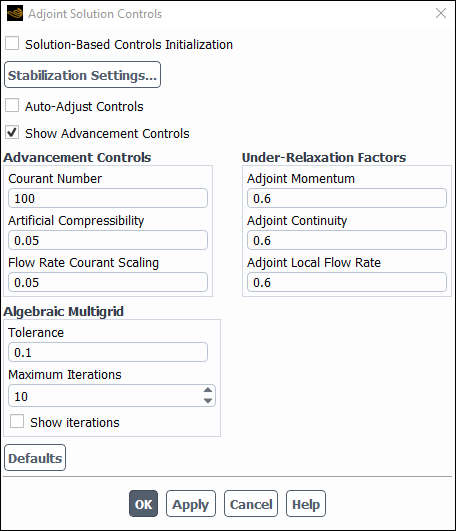
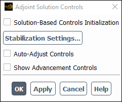
Open the Adjoint Solution Controls dialog box (Figure 30.6: Adjoint Solution Controls Dialog Box).
Design → Gradient-Based
→ Solver Controls...
Disable the Auto-Adjust Controls option.
This prevents Fluent from automatically choosing and adjusting the solution controls for you.
Enable Show Advancement Controls.
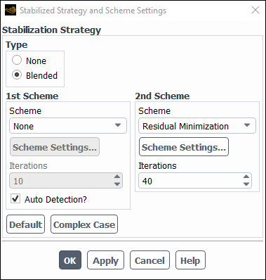
Select and enable Auto Detection?.
Click and then to close the dialog box.
Enter
100for Courant Number.Higher Courant Number values correspond to more aggressive settings / faster convergence, which is appropriate for a simple case such as this.
Enter
0.05for Artificial Compressibility.Click and then to close the dialog box.
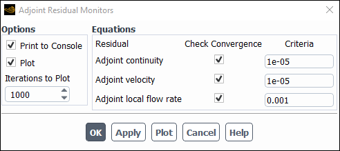
Configure the adjoint solution monitors by opening the Adjoint Residual Monitors dialog box (Figure 30.8: Adjoint Residual Monitors Dialog Box).
Design → Gradient-Based
→ Monitors...
In the Adjoint Residual Monitors dialog box, you set the adjoint equations that will be checked for convergence, as well as set the corresponding convergence criteria.
Make sure that the Print to Console and Plot options are enabled.
Enter values of
1e-05for Adjoint continuity and Adjoint velocity, and keep the default value of0.001for Adjoint local flow rate. These settings are adequate for most cases. Make sure that the Check Convergence options are enabled.Click and then to close the dialog box.
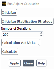
Run the adjoint solver using the Run Adjoint Calculation dialog box (Figure 30.9: Run Adjoint Calculation Dialog Box).
Design → Gradient-Based
→ Calculate...
Click the button. This initializes the adjoint solution everywhere in the problem domain to zero.
Set the Number of Iterations to
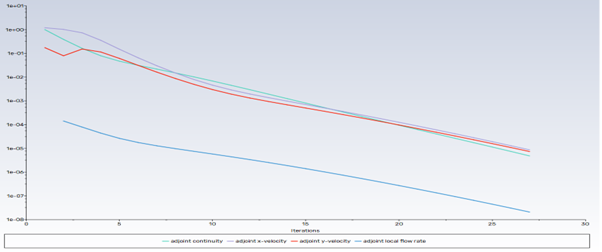
200. The adjoint solver is fully configured to start running for this problem.Click the button to advance the solver to convergence.
When the calculation is complete, the Run Adjoint Calculation dialog box.
In this section, postprocessing options for the adjoint solution are presented.
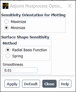
Open the Adjoint Postprocess Options dialog box.
Design → Gradient-Based
→ Postprocess Options...
Select Minimize from the Sensitivity Orientation for Plotting group box, because you are trying to reduce the drag force. This indicates that postprocessed results for the drag sensitivity will be displayed such that a reduction in drag is achieved by a design change in the positive sensitivity direction.
Click to apply the sensitivity orientation, then click to close the Adjoint Postprocess Options dialog box.
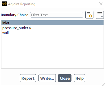
Open the Adjoint Reporting dialog box (Figure 30.12: Adjoint Reporting Dialog Box).
Design → Gradient-Based
→ Reporting...
Select inlet under Boundary Choice and click the button to display a report in the console of the available scalar sensitivity data on the inlet:
Updating shape sensitivity data.
Done.

Boundary condition sensitivity report: inlet
Observable: force-drag
Velocity Magnitude [m/s]: 40  Sensitivity ([N]/[m/s]): 54.55674
Decrease Velocity Magnitude to decrease force-drag
Close the Adjoint Reporting dialog box.
Open the Contours dialog box.
Results → Graphics
→ Contours → New...
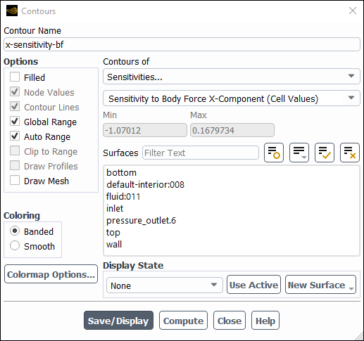
Enter
x-sensitivity-bffor the Contour Name.Disable Filled in the Options group.
Select Sensitivities... and Sensitivity to Body Force X-Component (Cell Values) from the Contours of drop-down lists.
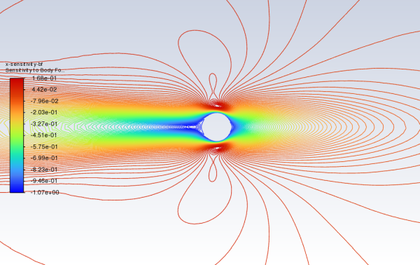
Click and then to view the contours (Figure 30.14: Adjoint Sensitivity to Body Force X-Component Contours) and then the Contours dialog box.
Figure 30.14: Adjoint Sensitivity to Body Force X-Component Contours shows how sensitive the drag on the cylinder is to the application of a body force in the
 -direction in the flow. If a body force is applied directly upstream
of the cylinder, for example, the disturbed flow is incident on the cylinder and
modifies the force that it experiences.
-direction in the flow. If a body force is applied directly upstream
of the cylinder, for example, the disturbed flow is incident on the cylinder and
modifies the force that it experiences.
Open the Vectors dialog box (Figure 30.15: Vectors Dialog Box)
Results → Graphics
→ Vectors → New...
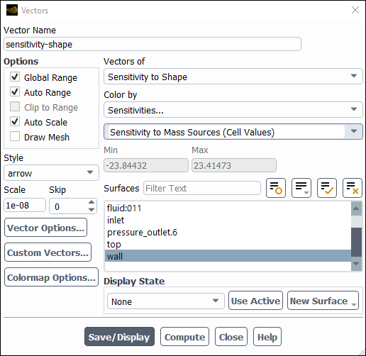
Enter
sensitivity-shapefor the Vector Name.Select Sensitivity to Shape from the Vectors of drop-down list.
Select Sensitivities... and Sensitivity to Mass Sources (Cell Values) from the Color by drop-down lists.
Select arrow from the Style selection list.
Enter
1e-8for Scale.Select wall from the Surfaces selection list.
Click the button to view the vectors (Figure 30.16: Shape Sensitivity Colored by Sensitivity to Mass Sources (Cell Values)) and then the Vectors dialog box.
Tip: In order to display the vector plot in the graphics window, you may need to click the Fit to Window button
 .
.
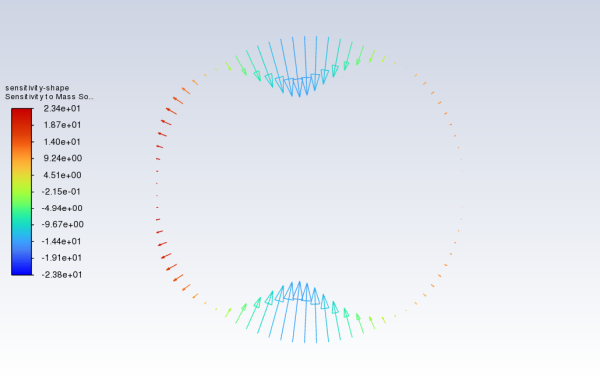
This plot shows how sensitive the drag on the cylinder is to changes in the surface shape. The drag is affected more significantly if the cylinder is deformed on the upstream rather than the downstream side. Maximum effect is achieved by narrowing the cylinder in the cross-stream direction.
Before computing the sensitivity for the force-lift observable, you need to define the region that will be subject to geometry morphing, and export the drag sensitivity data so it can be used later in the multi-objective optimization.
Open the Design Tool dialog box.
Design → Gradient-Based
→ Design Tool...
In the Region tab, define the region that will be modified for the design change.
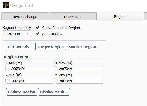
Ensure that Cartesian is selected from the Region Geometry drop-down list.
Click .
Select wall in the Bounding Region Definition dialog box and click OK.
This will initialize the morphing region to the bounding box around the cylinder wall.
Click to update the view of the bounding box illustration in the graphics window.
You can use the Mesh Display dialog box to also display the mesh, in order to review it prior to morphing.
Results → Graphics
→ Mesh → new...
Click Save/Display and close the Mesh Display dialog box.
Click several times until the X and Y Limits are ±1.907349 m (Figure 30.18: Morphing Region Around Cylinder).
In the Objectives tab, click Manage Data....
In the Manage Sensitivity Data dialog box, click and save the sensitivity data as
force-drag.sens.Close the Design Tool dialog box.
Select force-lift as the observable to be computed.
Design
→ Gradient-Based
→ Observable...
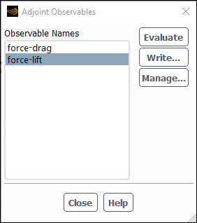
Select force-lift from the list of Observable Names, then click to close the Adjoint Observables dialog box.
Initialize and Calculate the adjoint solution using the Run Adjoint Calculation dialog box to obtain the sensitivities for the force-lift observable.
Design → Gradient-Based
→ Calculate...
Click Yes in the Question dialog box that appears to overwrite the existing adjoint solution data.
When the calculation is complete, you can optionally specify Maximum for the Sensitivity Orientation for Plotting similarly to Drag Force Sensitivity Orientation for Plotting. However for this example we will not be plotting the sensitivities for the force-lift observable and it is not necessary to define the sensitivity orientation for plotting. Additionally, you can export the sensitivity data for the lift observable as you did for the drag, but it is not strictly necessary if you plan to perform the multi-objective optimization in the current Fluent session.
In this section, you will load the previously saved force-drag sensitivity data and perform the multi-objective design change.
Open the Design Tool dialog box if it is not already open.
Design → Gradient-Based
→ Design Tool...
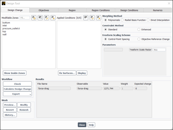
force-lift is now displayed in the Design Change tab because it is the currently selected observable. The Design Change tab functions as a dashboard for the design modification, where you can select which boundaries are subject to modification, enable or disable conditions that you have defined, specify relative weighting if you have multiple freeform objectives, and view predicted results. You will return to it to perform the design change after you have configured the objectives and the morphing region.
Retain the default selection of Polynomials from the Morphing Method list.
This morphing method is appropriate when you prefer mesh quality over adherence to the design conditions. Alternatively if there are many design conditions present, Direct Interpolation is the recommended method. Finally, when mesh quality is preferred and there are some design conditions, Radial Basis Function is the recommended method.
Load the previously saved force-drag sensitivity data.
Open the Objectives tab.
The force-lift observable is already listed because Include current data is enabled.
Click to open the Manage Sensitivity Data dialog box.
Click and select the force-drag.sens file you created earlier. Click .
Close the Manage Sensitivity Data dialog box.
Define the objective for each observable.
For this example, you will seek a design change that increases the lift and results in a 10% reduction in drag.
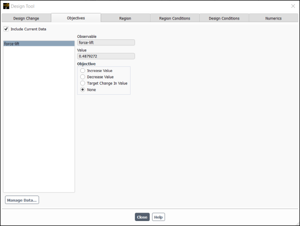
In the Objectives tab, select the force-lift observable. The current value of the lift is displayed along with options to specify the objective for the lift.
Select Increase Value from the Objective list.
This indicates that you want to increase the lift, but are not prescribing a specific target change.
Enter
100for Target/Reference Change.This setting is used to normalize the scale of the change in value of the observable, which can be important in cases where multiple observables are considered that may be of different scales.

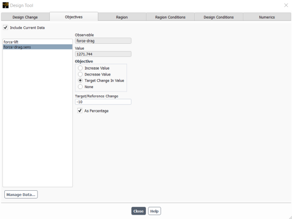
Select force_drag.sens in the list of observables.
Select Target Change In Value from the Objective list.
This indicates that you are prescribing a specific change in the value of the observable, rather than a freeform increase or decrease.
Enter
-10for Target/Reference Change and enable the As Percentage option.10% is a generally a reasonable maximum target change for a design change. Using a target change that is too large may result in very large deformations and/or overshooting the local optimum.
Configure the morphing region.
You already specified the dimensions of the region earlier when exporting the force-drag sensitivity. Now you will also configure the control-point density.
Click the Region Conditions tab in the Design Tool dialog box.
Enter
30for Points in the In X Direction and In Y Direction group boxes.You can use the Mesh Display dialog box to display the mesh, in order to see the increase in control points.
Results → Graphics
→ Mesh → New... Many other settings are available in the Region Conditions tab, including constraints on control-point motion, symmetry conditions, and continuity conditions. For additional information, see the section on defining region conditions in the Fluent User's Guide manual.
Compute the design change and modify the mesh.
Return to the Design Change tab.
Select wall in the Modifiable Zones selection list.
Only zones that are selected in the Modifiable Zones list (or that have prescribed motions applied) will be modified as part of the design change.
If multiple freeform objectives were defined (that is, multiple objectives with Increase Value or Decrease Value selected in the Objectives tab), you would need to specify the Weight for each. In this case only one objective (force-lift) is freeform, so no input is required for Weight.
Retain the default settings of Control-Point Spacing for Freeform Scaling Scheme, and 0.1 for Freeform Scale Factor.
These settings allow you to adjust the magnitude of the attempted design change (Freeform Scale Factor) and the basis for the scaling (Freeform Scaling Scheme).
Click .
The Results list is updated to reflect the Expected change for each observable.
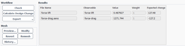
Note that the drag is predicted to decrease by 10% as you requested, and the lift is predicted to increase.
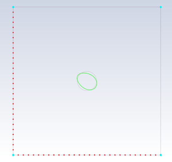
Click the button in the Mesh group box to preview the design change in the graphics window.
Select
wallon the Preview Morphing dialog box and click Display.Click OK in the Warning dialog box that appears.
Click the button in the Mesh group box to apply the calculated mesh deformation that will reposition the boundary and interior nodes of the mesh. Information regarding the mesh modification is printed in the console:
Updating mesh (steady, mesh iteration = 00001, pseudo time step 1.0000e+00)...
Dynamic Mesh Statistics:
Minimum Volume    = 3.24815e-04
Maximum Volume    = 6.36270e-01
Maximum Cell Skew = 3.75949e-01 (cell zone 11)
Minimum Orthogonal Quality = 6.24051e-01 (cell zone 11)
Display the new mesh geometry.
 Results → Graphics
→ Mesh → mesh-1
Results → Graphics
→ Mesh → mesh-1 Edit...
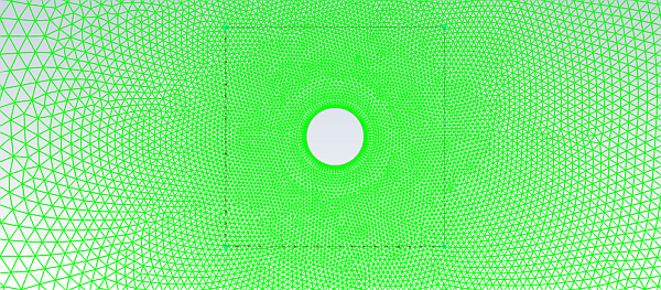
Click Save/Display and close the Mesh Display dialog box.
The effect on the mesh is shown in Figure 30.21: Mesh After Deformation:
Re-converge the conventional flow calculation for this new geometry in the Run Calculation task page.
Solution → Run
Calculation → Calculate
The currently loaded case file already has report definitions defined for lift and drag, or you can Evaluate the new values in the Adjoint Observables dialog box.
Design
→ Gradient-Based
→ Observable...
The new values for drag and lift are reported to be:
Observable name: force-drag
Observable Value [N]: 1151.1871


Observable name: force-lift
Observable Value [N]: 122.87626
Note that the drag has changed by -120.55 N or -9.5% compared to the drag on the undeformed cylinder. This value compares very well with the change of -127.2 N (-10%) that was predicted from the adjoint solver. The lift has increased by 294.4 N, which again compares very well with the predicted change of 291.91 N.
Save the case and data files (
cylinder-adjoint.cas.h5andcylinder-adjoint.dat.h5). File → Write →
Case & Data...

This tutorial has demonstrated how to use the adjoint solver to compute the sensitivity of the drag and lift on a circular cylinder to various inputs for a previously computed flow field. The process of setting up and running the adjoint solver was illustrated. The steps to perform various forms of postprocessing were also described. The design change tool was used to make a multi-objective change to the design that reduced the drag and increased the lift in a predictable manner.
This example considered multiple objectives at a single flow condition. Another powerful application of the design tool is to perform multi-objective design changes using sensitivities computed for multiple flow conditions. This allows you to identify design changes that improve performance across a range of anticipated operating conditions, potentially of differing importance. The design tool also offers a rich set of additional capabilities for including prescribed deformations, bounding planes / surfaces, and fixed-wall constraints in your multi-objective design change.