Chapter 27: Modeling Ablation

This tutorial is divided into the following sections:

27.1. Introduction

In this tutorial, a flow field of air passing around a 3D wedge is simulated using the Ansys Fluent ablation mode. Ablation is an effective treatment used to protect a vehicle from the damaging effects of external high temperatures. During high speed vehicle operations (for example, vehicle reentry), the ablative coating is chipped away to remove excessive amount of heat from the surface of the vehicle.

This tutorial demonstrates how to do the following:

Define boundary conditions for a high-speed flow.
Set up the ablation model to model effects of a moving boundary due to ablation.
Initiate and solve the transient simulation using the density-based solver.

27.2. Prerequisites

This tutorial is written with the assumption that you have completed the introductory tutorials found in this manual and that you are familiar with the Ansys Fluent outline view and ribbon structure. Some steps in the setup and solution procedure will not be shown explicitly.

27.3. Problem Description

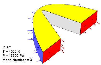
The geometry of the 3D wedge considered in this tutorial is shown in Figure 27.1: Problem Schematic. The air flow passes around a nose of a re-entry vehicle operating under high speed conditions. The inlet air has a temperature of 4500 K, a gauge pressure of 13500 Pa, and a Mach number of 3. The domain is bounded above and below by symmetry planes (displayed in yellow). As the ablative coating chips away, the surface of the wall moves. The moving of the surface is modeled using dynamic meshes. The surface moving rate is estimated by Vielle’s empirical law:

where is the surface moving rate, is the absolute pressure, and and are model parameters. In the considered case, = 5 and = 0.1.

Figure 27.1: Problem Schematic

27.4. Setup and Solution

The following sections describe the setup and solution steps for this tutorial:

27.4.1. Preparation

To prepare for running this tutorial:

Download the ablation.zip file here .
Unzip ablation.zip to your working directory.
The mesh file ablation_mesh.msh can be found in the folder.
Use the Fluent Launcher to start Ansys Fluent.
Select Solution in the top-left selection list to start Fluent in Solution Mode.
Select 3D under Dimension.
Enable Double Precision under Options.
Set Solver Processes to 4 under Parallel (Local Machine).

27.4.2. Mesh

Read the mesh file ablation.msh.h5.
File → Read → Mesh...
Check the mesh.
Domain → Mesh → Check → Perform Mesh Check
Ansys Fluent will perform various checks on the mesh and report the progress in the console. Ensure that the reported minimum volume is a positive number.
Display the mesh.
Domain → Mesh → Display...
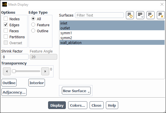
1. In the Options group box, disable Faces and enable Edges.
2. From the Surfaces selection list, select inlet, outlet, and wall-ablation.
  Tip: To deselect all surfaces click the far-right button at the top of the Surfaces selection list, and then select the desired surfaces from the Surfaces selection list.
3. In the Edge Type group box, ensure that All is selected.
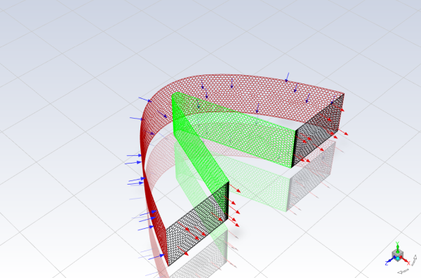
4. Click Display and close the Mesh Display dialog box.
The graphics display will be updated to show the mesh (see Figure 27.2: Wedge Mesh Display). The inlet is colored blue, the walls are colored gray, the symmetry planes are colored yellow, and the outlet is colored red.
Figure 27.2: Wedge Mesh Display

27.4.3. Solver

In the General task page, retain the default solver settings of Denisty-Based solver type.
Setup → General → Density-Based
The density-based solvers of Ansys Fluent provides faster performance for applications involving high-speed aerodynamics with shocks.
Select Transient from the Time list.
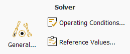
Setup → General → Transient
Set the Operating Conditions.
Physics → Solver → Operating Conditions...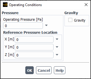
1. Enter 0 for Operating Pressure.
2. Click OK to confirm the operating conditions.

27.4.4. Models

Enable heat transfer by enabling the energy equation.
Physics → Models → Energy
Enable the k-ω SST turbulence model.
Physics → Models → Viscous...
1. Retain the default selection of k-omega (2 eqn) in the Model list.
2. Retain the default selection of SST in the k-omega Model list.
3. Click OK to close the Viscous Model dialog box.
Enable the ablation model.
Physics → Models → More... → Ablation...
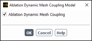
1. In the Ablation Dynamic Mesh Coupling Model dialog box, enable Ablation Dynamic Mesh Coupling.
2. Click OK to close the Ablation Dynamic Mesh Coupling Model dialog box.

27.4.5. Materials

The default Fluid Material is air, which is the working fluid in this problem. The default settings need to be modified to account for compressibility.

Set the properties for air, the default fluid material.
Setup → Materials → Fluid → air Edit...
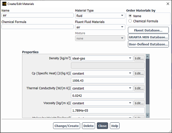
1. In the Properties group, select ideal-gas from the Density drop-down list.
2. Click Change/Create to save these settings.
3. Close the Create/Edit Materials dialog box.

27.4.6. Boundary Conditions

Specify boundary conditions using the Boundary Conditions task page.

Setup → Boundary Conditions

Set the boundary conditions for the air inlet (inlet).

Setup → Boundary Conditions → inlet

In the Boundary Conditions task page, select inlet from the Zone list.
From the Type drop-down list, select pressure-far-field.
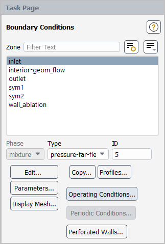
Click Edit... to open the Pressure Far-Field dialog box.

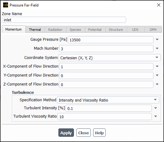
In the Pressure Far-Field dialog box, configure the following settings:

Tab	Setting	Value
Momentum	Gauge Pressure	`13500` Pa
	Mach Number	`3`
	Specification Method	Intensity and Viscosity Ratio (default)
	Turbulent Intensity	`0.1` %
Thermal	Temperature	`4500` K

Click Apply and close the Pressure Far-Field dialog box.

Set the boundary conditions for the air outlet (outlet).

Setup → Boundary Conditions → outlet → Edit...

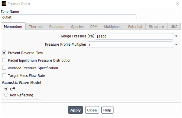
In the Pressure Outlet dialog box, configure the following settings:

Tab	Setting	Value
Momentum	Gauge Pressure	`13500` Pa
Momentum	Prevent Reverse Flow	(Selected)

Click Apply and close the Pressure Outlet dialog box.

Set the ablation boundary conditions for the wall (wall_ablation).

Setup → Boundary Conditions → wall_ablation → Edit...

In the Wall dialog box, configure the following settings:

Tab	Setting	Value
Ablation	Ablation Model	Vielle’s Model
	Parameter A	`5`
	Parameter n	`0.1` (default)

Click Apply and close the Wall dialog box.
Once you have specified the ablation boundary conditions for the wall, Ansys Fluent automatically enables the Dynamic Mesh model with the Smoothing and Remeshing options, creates the wall-ablation dynamic mesh zone, and configure appropriate dynamic mesh settings.

27.4.7. Dynamic Mesh

For ablation simulations, you must define dynamic mesh zones to allow the mesh to handle the zone deformation in the Dynamic Mesh... task page.

Domain → Mesh Models → Dynamic Mesh...

In the Mesh Methods group box, click the Settings... button to open the Mesh Method Settings dialog box.
Review and retain the current settings for smoothing and remeshing.
Note: In general, there is no need to modify the dynamic mesh settings automatically configured by Ansys Fluent. However, you can adjust these settings to suit your specific needs.
Click OK to close the Mesh Method Settings dialog box.
Click the Create/Edit... button to open the Dynamic Mesh Zones dialog box.
Create the dynamic zone for the fluid cell zone.
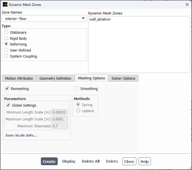
1. From the Zone Names drop-down list, select interior--flow.
2. From the Type list, select Deforming.
3. In the Meshing Options tab, disable Smoothing.
4. Retain the remaining default settings and click Create.
Create the dynamic zone for the outlet.
1. From the Zone Names drop-down list, select outlet.
2. From the Type list, select Deforming.
3. In the Meshing Options tab, enable Smoothing.
4. Retain the remaining default settings and click Create.
Create the dynamic zones for the symmetry zones.
1. From the Zone Names drop-down list, select symm1.
2. From the Type list, select Deforming.
3. In the Meshing Options tab, enable Smoothing.
4. In Geometry Definition tab, select plane from the Definition drop-down list.
5. In the Point on Plane group box, enter 0, -0.04, and 0 for X, Y, and Z.
6. In the Plane Normal group box, enter 0, -1, and 0 for X, Y, and Z.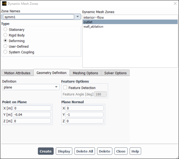
7. Click Create.
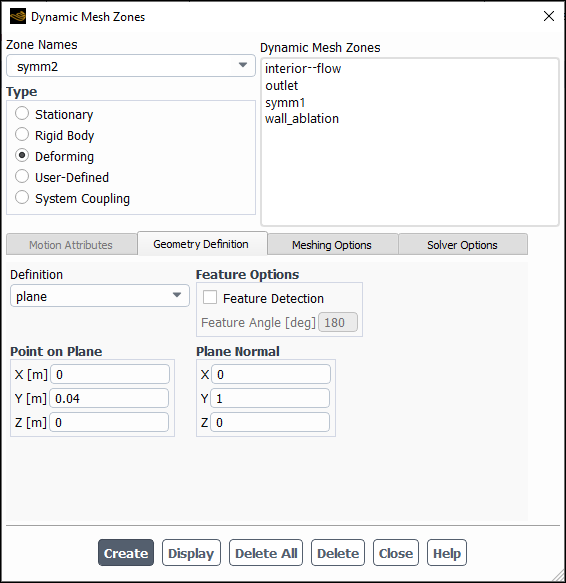
8. In a similar manner, create the dynamic zone for symm2. For the Point on Plane, enter 0, 0.04, and 0 for X, Y, and Z, respectively. For the Plane Normal, enter 0, 1, and 0 for X, Y, and Z, respectively.
  Click Create.
Enable the movement of the adjacent boundary layer mesh with the moving face zone for the wall_ablation dynamic zone.
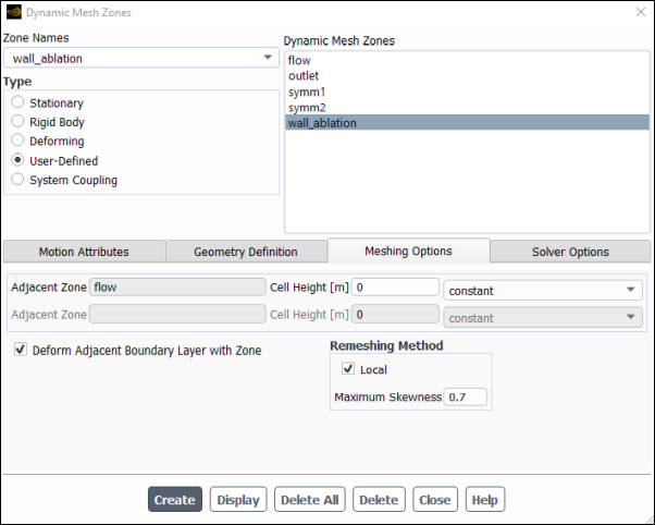
1. From the Zone Names drop-down list, select wall_ablation.
2. From the Type list, select User-Defined.
3. In the Meshing Options tab, enable Deform Adjacent Boundary Layer with Zone.
4. Click Create and close the Dynamic Mesh Zones dialog box.

27.4.8. Solution

Set the solution methods.
Solution → Solution → Methods...
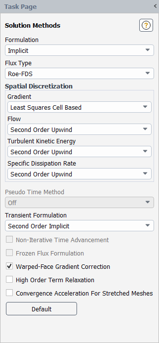
1. Retain the selection of Implicit and Roe-FDS from the Formulation and Flux Type drop-down lists, respectively.
2. For the Gradient spatial discretization, select Least Squares Cell Based.
3. Retain the default selections of Second Order Upwind for the remaining spatial discretizations.
4. From the Transient Formulation drop-down list, select Second Order Implicit.
5. Enable the Warped-Face Gradient Correction option.
In the Solution Controls task page, adjust the solution settings.
1. Retain the under-relaxation factors.
2. Click Limits... to open the Solution Limits dialog box.
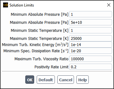
3. Enter 25000 K for the Maximum Static Temperature.
4. Click OK to close the Solution Limits dialog box.
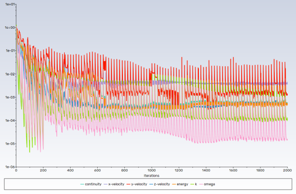
Enable the plotting of residuals during the calculation.
Solution → Reports → Residuals...
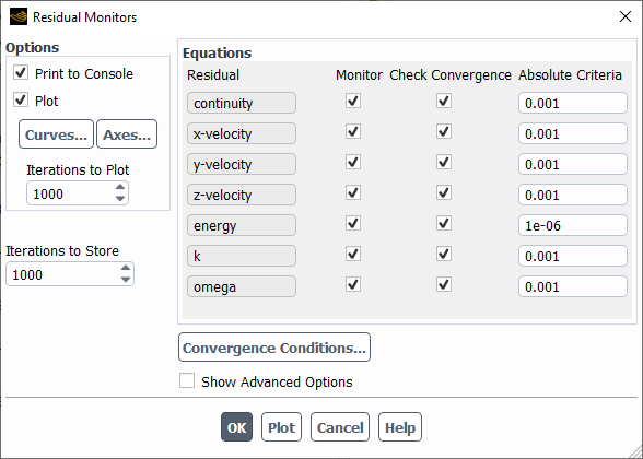
1. Ensure that Plot is enabled in the Options group box.
2. Enter 1e-06 for energy and retain the default values for the Absolute Criteria of continuity, x-velocity, y-velocity, z-velocity, k, and omega.
3. Click OK to close the Residual Monitors dialog box.
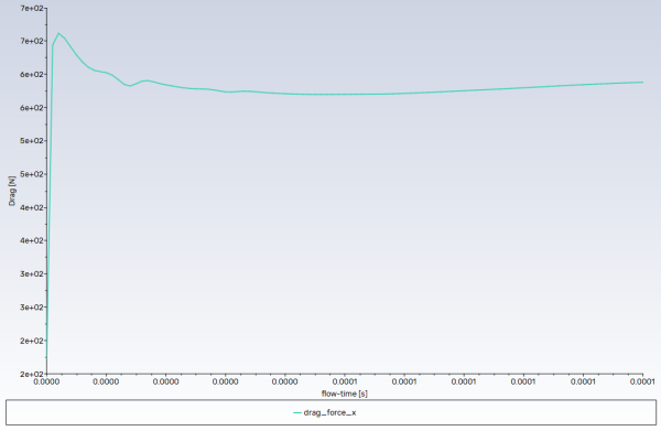
Create a force report definition to plot and write the drag force on the wall_ablation wall boundary.
Solution → Reports → Definitions → New → Force Report → Drag...
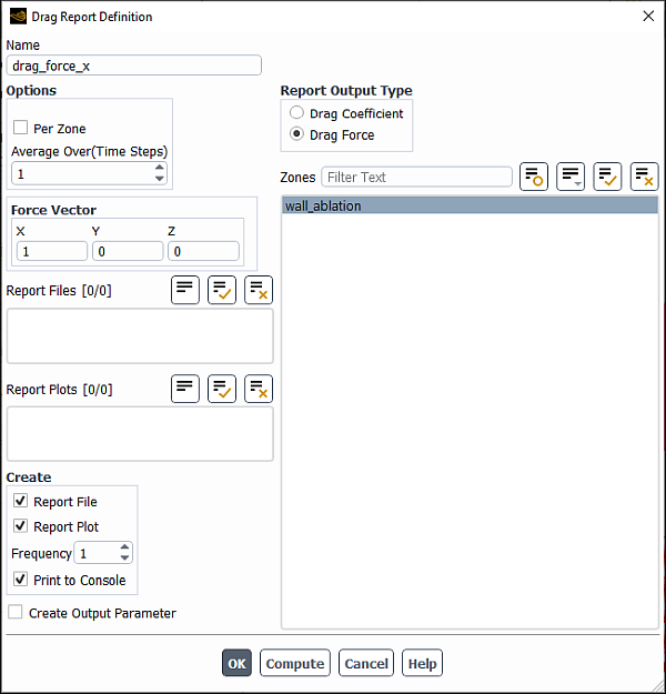
1. In the Drag Report Definition dialog box, enter drag_force_x for Name.
2. Select Drag Force in the Report Output Type list.
3. Select wall_ablation from the Wall Zones list.
4. In the Create group box, enable Print to Console.
5. Click OK to create the report.
  Fluent automatically generates the drag_force_x-rplot report plot under Solution/Monitors/Report Plots tree branch and the drag_force_x-rfile report file under Solution/Monitors/Report Files tree branch.
6. Modify the attributes of the drag_force_x-rplot report plot axes.
  Solution → Monitors → Report Plots → drag_force_x-rplot Edit...
  1. In the Edit Report Plots dialog box, click the Axes... button to open the Axes - Report Plots dialog box.
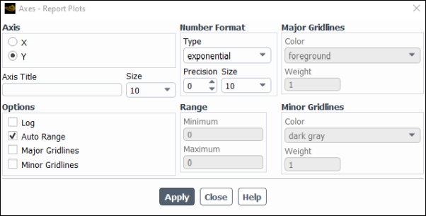
  2. In the Axis list, select Y.
  3. Select exponential from the Type drop-down list.
  4. Set Precision to 0.
  5. Click Apply to save the modified settings and close the Axes - Report Plots dialog box.
  6. Click OK to close the Edit Report Plot dialog box.
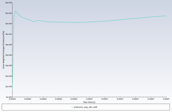
Create a surface report definition for the averaged pressure at the wall_ablation boundary.
Solution → Reports → Definitions → New → Surface Report → Area-Weighted Average...
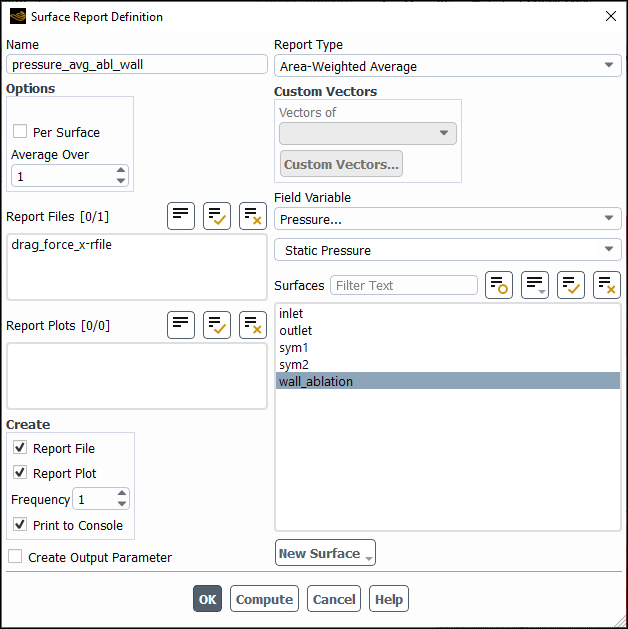
1. In the Surface Report Definition dialog box, enter pressure_avg_abl_wall for Name.
2. Retain Pressure... and Static Pressure from the Field Variable drop-down lists.
3. From the Surfaces selection list, select wall_ablation.
4. In the Create group box, enable Print to Console.
5. Click OK to save the surface report definition and close the Surface Report Definition dialog box.
6. Modify the attributes of the pressure_avg_abl_wall-rplot report plot axes in a manner similar to that for the drag_force_x-rplot plot.
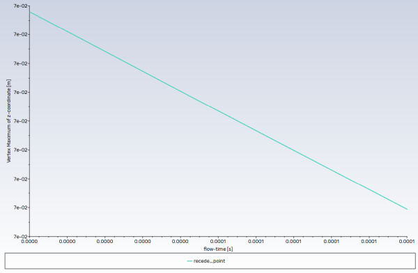
Create a surface report definition for the maximum value of the Z-coordinate at the wall_ablation boundary to monitor the effects of the mesh movement.
Solution → Reports → Definitions → New → Surface Report → Vertex Maximum...
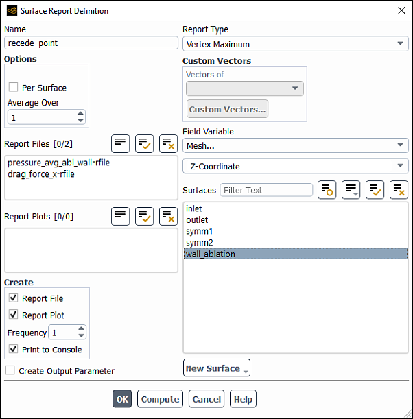
1. In the Surface Report Definition dialog box, enter recede_point for Name.
2. Select Mesh... and Z-Coordinate from the Field Variable drop-down lists.
3. From the Surfaces selection list, select wall_ablation.
4. In the Create group box, enable Print to Console.
5. Click OK to save the surface report definition and close the Surface Report Definition dialog box.
6. Modify the attributes of the recede_point-rplot report plot axes in a manner similar to that for the drag_force_x-rplot plot.
Initialize the flow field.
Solution → Initialization → Options...
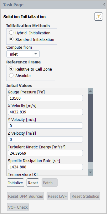
1. In the Solution Initialization task page, select the Standard Initialization from the Initialization Methods group.
2. Select inlet from the Compute from drop-down list.
3. Click Initialize to initialize the variables.
Save the case file (ablation.cas.h5).
File → Write → Case...
Run the calculation.
Solution → Run Calculation → Run Calculation...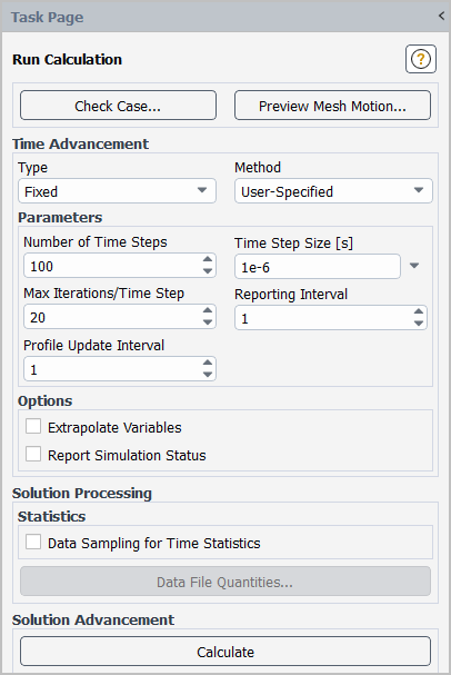
1. Enter 100 for Number of Time Steps.
2. Enter 1e-6 for Time Step Size.
3. Click Calculate.
  Note: It may take significant time and computer resources to complete the problem calculation.
  Figure 27.3: Scaled Residuals
  
  Figure 27.4: History of the Drag Force on the Ablation Wall
  
  Figure 27.5: History of the Averaged Pressure on the Ablation Wall
  
  Figure 27.6: History of the Maximum Z Coordinate of the Ablation Wall
Save the case and data files (ablation.cas.h5 and ablation.dat.h5).
File → Write → Case & Data...

27.4.9. Postprocessing

Create an iso-surface through the domain geometry.
Results → Surface → Create → Iso-Surface...
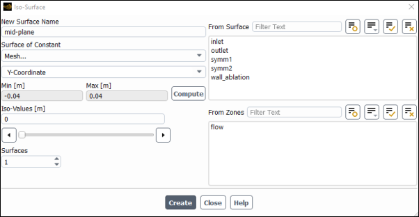
1. Enter mid_plane for the New Surface Name.
2. Select Mesh... and Y-Coordinate from the Surface of Constant drop-down lists.
3. Click Compute to update the minimum and maximum values.
4. Retain the value of 0 for Iso-Values.
5. Click Create and then close the Iso-Surface dialog box.
Display static pressure contours on the mid_plane iso-surface. (Figure 27.7: Contours of Static Pressure).
This will allow you to review the location of the droplets.
Results → Graphics → Contours → New...
1. Enter contour-pressure for Contour Name.
2. Ensure that Filled is enabled in the Options group box.
3. Retain the selection of Smooth in the Coloring group box.
4. Retain the default selection of Pressure... and Static Pressure from the Contours of drop-down lists.
5. Select mid_plane from the Surfaces selection list.
6. Click Save/Display and close the Contours dialog box.
  Figure 27.7: Contours of Static Pressure
  
  Note that the static pressure near the tipping point of the wedge has the highest value, as expected.
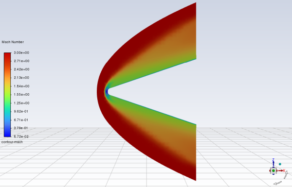
Display contours of the Mach number on the mid_plane iso-surface. (Figure 27.8: Contours of Mach Number).
This will allow you to review the location of the droplets.
Results → Graphics → Contours → New...
1. Enter contour-mach for Contour Name.
2. Ensure that Filled is enabled in the Options group box.
3. Retain the selection of Smooth in the Coloring group box.
4. Select Velocity… and Mach number from the Contours of drop-down lists.
5. Select mid_plane from the Surfaces selection list.
6. Click Save/Display and close the Contours dialog box.
  Figure 27.8: Contours of Mach Number
  
  In Figure 27.8: Contours of Mach Number, you can observe an oblique shock formed in the domain. The Mach number (or velocity) is the lowest at the tipping point of the wedge where the static pressure is the highest (see Figure 27.7: Contours of Static Pressure).
Save the case and data files (ablation.cas.h5 and ablation.dat.h5).
File → Write → Case & Data...

27.5. Summary

In this tutorial, you used the Ansys Fluent ablation model to predict the ablation effects in a 3D wedge flow. The Vielle's model was used to model the surface recession rate. The procedures used here can be applied to other applications that involve ablation modeling.